Tracing ice loss from the Late Holocene to the future in eastern Nuussuaq, central western Greenland

Greenland's peripheral glaciers and ice caps (GICs) have experienced accelerated mass loss since the 1990s. However, the extent to which projected future trends in GICs are unprecedented within the Holocene is poorly understood. This study bridges the gap between the maximum ice extent (MIE) of the Late Holocene and present and future glacier evolution until 2100 in the eastern Nuussuaq Peninsula (central western Greenland). The Instructed Glacier Model (IGM) is calibrated and validated by simulating present-day glacier area and ice thickness. The model is employed to reconstruct the eastern Nuussuaq Peninsula GICs to align with the MIE of the Late Holocene, which occurred during the late Medieval Warm Period (1130±40 and 925±80 CE), based on moraine boulder surface exposure dating from previous studies. Subsequently, the model is forced with CMIP6 projections for SSP2–4.5 and SSP5–8.5 scenarios (2020–2100). The Late Holocene MIE is reached when temperatures decrease by ≤1 °C relative to the baseline climate (1960–1990) using a calibrated melt rate factor. Currently, the glaciated area and ice thickness have declined by 15±5 % compared to the MIE, with the standard deviation (±) reflecting the influence of the calibrated and low-end melt rate factors. By 2100, temperatures are projected to rise by up to 6 °C (SSP5–8.5) above the baseline, exceeding Holocene Warm Period (∼10 to 6 ka) levels by a factor of 3. Ice loss is expected to accelerate rapidly, reaching $-\mathrm{56}\pm \mathrm{6}$ % relative to present-day levels by 2070–2080 (SSP5–8.5), with near-total glacier disappearance projected by 2090–2100. This study contextualizes present and future glacier retreat within a geologic timescale and quantifies the impacts of anthropogenic climate change on the cryosphere.

1 Introduction

Arctic temperatures are rising at a faster (∼4 times) rate than the global average (Rantanen et al., 2022), and glaciers are displaying accelerated ice loss (Hugonnet et al., 2021). In 2021, Greenland's peripheral glaciers and ice caps (GICs) represented a small (4 %) ice cover area of the island but contributed to 11 % of the total Greenland ice loss and sea level rise (Khan et al., 2022). The recession of glaciers implies alterations in fauna and flora patterns (Saros et al., 2019), as well as impacts on water availability, climate, and ocean and atmospheric dynamics that have environmental and climate consequences far beyond the polar regions (IPCC, 2022).

The Little Ice Age (LIA; 1300–1900 CE) has been defined as the last period with widespread glacier expansion (Kjær et al., 2022). Greenland GICs lost 499 Gt of ice from the end of LIA to 2021 (Carrivick et al., 2023). The rate of loss of GICs has increased since the 1990s (Bolch et al., 2013; Larocca et al., 2023), with recent trends indicating an acceleration in mass loss from 27.2±6.2 Gt yr⁻¹ (February 2003–October 2009) to 42.3±6.2 Gt yr⁻¹ (October 2018–December 2021) (Khan et al., 2022). Warming rates have been higher in western Greenland than in the east since the end of the LIA (Hanna et al., 2012). As a result, the loss of ice from Greenland's GICs has been more pronounced at the country's western fringe, where warmer conditions have been associated with the positive phase of the North Atlantic Oscillation (NAO), resulting in a west-to-east warming gradient (Bjørk et al., 2018). Historical records reveal varying trends in GICs over the past 2 centuries. Aerial images and satellite data indicate that GICs in western Greenland remained relatively stable, maintaining their extent from the middle of the 19th century until the middle of the 20th century, after which they experienced rapid retreat (Weidick, 1994; Leclercq et al., 2012). For instance, Citterio et al. (2009) observed a reduction in glacier area of approximately 20 % from the LIA to 2001. Other estimates suggest a 48 % loss in GIC area in southern western Greenland from the maximum extent of the LIA until 2019 (Brooks et al., 2022).

The recent evolution of the GICs has been reconstructed using historical aerial images and satellite records (Leclercq et al., 2012; Yde and Knudsen, 2007; Citterio et al., 2009; Bjørk et al., 2018; Larocca et al., 2023). Geospatial techniques, such as the inference of the equilibrium line altitude (ELA), have also been utilized (Brooks et al., 2022; Carrivick et al., 2023). However, aerial and satellite images provide temporal data over centuries and decades, and geospatial methods neglect ice flow physics and do not account for glacier dynamics. Based on the distribution of moraines and unvegetated trimlines in central western Greenland, some authors suggested that the Late Holocene maximum glacier extent occurred around the LIA (Humlum, 1999). However, cosmic ray exposure (CRE) dating of erosive and depositional glacial records indicates that the maximum ice extent (MIE) of the Late Holocene did not occur during the LIA in many areas in western Greenland but rather during the Medieval Warm Period (MWP; 950 to 1250 CE) (Young et al., 2015; Jomelli et al., 2016; Schweinsberg et al., 2019).

Compared to studies near the Greenland Ice Sheet (GrIS) (e.g., Cuzzone et al., 2019; Briner et al., 2020), there is limited evidence from physically based models regarding the GIC recession during the Holocene. Holocene reconstructions of GrIS extent based on physical modeling, guided by geomorphological evidence, provide valuable insights into the paleoclimate conditions that led to the MIE of the Late Holocene and the subsequent recession (Simpson et al., 2009; Lecavalier et al., 2014; Cuzzone et al., 2019), facilitating comparisons of past and future glacier responses to climate change (Briner et al., 2020). Physically based ice flow modeling relying on full Stokes equations are computationally intensive at high resolutions (sub-kilometer) for long-term paleo glacier simulations and model parameter calibrations (Jouvet et al., 2022). Simplified models such as the hydrostatic shallow-ice approximation (SIA) and the shallow-shelf approximation (SSA) tend to overestimate ice velocities near glacier margins and underestimate velocities in deep glaciated areas. An emulator based on a convolutional neural network (CNN), trained with high-order ice flow equations, offers reduced computational costs while maintaining accurate ice thickness estimates comparable to those obtained through high-order equations (Jouvet, 2023; Jouvet et al., 2023).

The future recession of Greenland GICs compared to the long-term Holocene fluctuations is poorly understood. Here, we calibrate and validate the Instructed Glacier Model (IGM) (Jouvet, 2023), a glacier evolution model based on a CNN emulator used to estimate ice flow, to reconstruct the MIE of the Late Holocene in an extended glacier area in the eastern Nuussuaq Peninsula (central western Greenland). This area has CRE records available for the outermost glacier moraine complexes, but the paleoclimate conditions causing these glacier oscillations are not yet known in detail (D'andrea et al., 2011; Biette et al., 2018; Jomelli et al., 2016; Schweinsberg et al., 2019; Osman et al., 2021). Employing the IGM allows us to reconstruct glaciers in high (90 m) resolution based on high-order equations (Jouvet, 2023), demonstrating the methodology's capabilities for glacier modeling at regional scales. Future glacier evolution is modeled under the CMIP6 SSP2–4.5 and SSP5–8.5 scenarios, from present and steady-state glacier conditions to the year 2100. We compared the projected ice loss trend against the reconstructed MIE of the Late Holocene to the present-day ice loss trends, extending glacier records from decades to millennia and placing present and future glacier shrinkage within a long-term Holocene perspective.

The objectives of this work are to (i) reconstruct past glaciers under different climate conditions, (ii) determine past and future climate conditions influencing the MIE of the Late Holocene and future glacier recession, (iii) quantify future glacier retreat trends, and (iv) compare future ice loss trends with the rate of ice loss from the MIE of the Late Holocene to the present.

2 Study area

This study focuses on a land-terminating glacier area in the Nuussuaq Peninsula, central western Greenland (Fig. 1). This peninsula extends from the onshore Disko (south) to Svartenhuk Halvo (north). Nuussuaq Peninsula includes several mountain glaciers and ice caps connected to the GrIS that surrounds its eastern flank. Our study focuses on a glacier area in the eastern Nuussuaq Peninsula, with elevations ranging from 400 to 1200 m above sea level (m a.s.l.) (Fig. 1).

Present-day climate conditions are characterized by a polar maritime climate, becoming more continental toward the inland areas and the GrIS (Humlum, 1999). Moist air masses from the Davis Strait influence the climate during summer, with continental polar-air influences during the winter (Ingolfsson et al., 1990). Prevailing winds in the region typically come from the east and northeast, except during the summer months, when southerly and southwesterly winds prevail (Humlum, 1999). The relief configuration exposes Disko Bay to cyclogenic activity and moist airflow, resulting in decreased precipitation from the peripheral coastal areas towards the GrIS (Weidick and Bennike, 2007). The nearest research station with meteorological and snow observations is the Arctic station on the coastal Disko Island (central western Greenland). Here, the accumulated annual precipitation is 436 mm (1991–2004 period) (Hansen et al., 2006). The mean annual temperature (MAAT) is −4 °C (1961–1990 period), with a lapse rate of around 0.6 °C per 100 m (Humlum, 1998). At the Arctic station, the snow season typically extends from September to June, with maximum snow accumulations of around 50 cm (Bonsoms et al., 2024a).

The present-day landscape in central western Greenland is characterized by the presence of glaciers, which have also intensely shaped the relief in ice-free areas in the past. Today, environmental dynamics in these areas are strongly influenced by periglacial processes under a continuous permafrost regime (Humlum, 1998; Christiansen et al., 2010) that reshape the geological setting made of clastic sediments from the mid-Cretaceous to the Palaeogene (Pedersen et al., 2002). The strong glacial imprint in the landscape of the peninsula results from a complex glacial history, which is not yet known in detail. Following the Last Glacial Maximum (LGM), the GrIS underwent a significant retreat during Termination-1 and exposed the coastal regions in central western Greenland (Briner et al., 2020). As in other regions across Greenland, the Early Holocene was characterized by warm temperatures that led glaciers to retreat (Leger et al., 2024). In the Nuussuaq Peninsula, CRE records reported the onset of glacial retreat by ca. 10 ka (O'Hara et al., 2017). The minimum GrIS extension occurred from ca. 5 to 3 ka cal BP, when GrIS margins retreated by ca. 150 km from the present-day terminus position (Briner et al., 2020), which explains the lack of glacial records corresponding to the Early to Middle Holocene in the peninsula (Kelly and Lowell, 2009; O'Hara et al., 2017). According to several absolute dating methods in different natural records, the Nuussuaq Peninsula GICs grew between approximately 4.3 and 2 ka and reached several glacier culminations during the last millennium before the LIA (Schweinsberg et al., 2017, 2019). The internal and external moraine complexes in the area showed CRE ages of 1130±40 and 925±80 CE, respectively (Young et al., 2015). These ages are consistent with other CRE ages obtained in central western Greenland for the most external recent moraine complexes, indicating that the late MWP glacier expansion was the largest of the Late Holocene (Jomelli et al., 2016; Schweinsberg et al., 2019).

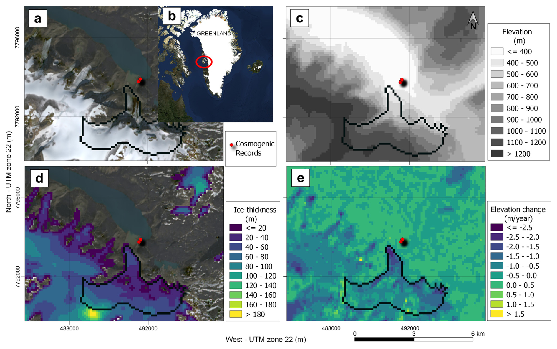
Figure 1 Location of the reconstructed glacier and CRE ages (red points) used in this work (a). Location of the study area within Greenland (b). Glacier delimitation is based on Randolph Glacier Inventory (RGI6). The base map is a Sentinel-2 image from https://s2maps.eu/ (last access: 7 May 2025; 2022). Elevation map of the study area from a Copernicus GLO-90 digital elevation model (2010–2015) (c). Average ice thickness (m) (2018–2022) from Millan et al. (2022) (d). Elevation changes in terms of average values (m yr⁻¹) between 2000–2019 (Hugonnet et al., 2021) (e).

3 Data

3.1 Pre-processing glacier data download

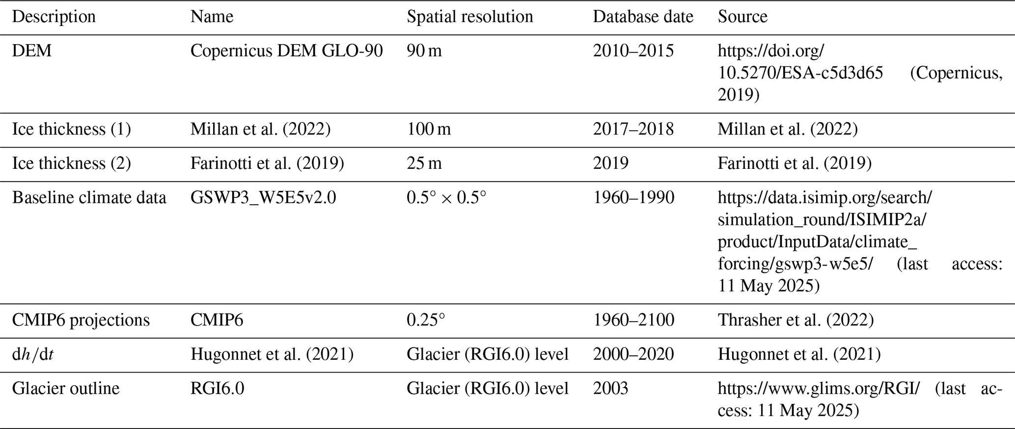
The data used to force and validate the IGM are detailed in Table 1. Topography data were obtained from a Copernicus digital elevation model (DEM) with a resolution of 90 m (Copernicus GLO-90). In situ mass balance records in the study area are scarce, and fieldwork is challenging. However, recent advancements in global-scale mass balance, satellite imagery, and ice thickness estimates have enabled the validation of the glacier model. We compared the ice thickness estimates from Farinotti et al. (2019), which constitute the outputs from an ensemble of five models (HF-model, GlabTop2, OGGM, GlabTop2 IITB version, and an unnamed model), with those from Millan et al. (2022), which are derived from numerical modeling based on SIA and data obtained from a constellation of remote sensing products (Sentinel-1/ESA, Sentinel-2/ESA, Landsat-8/USGS, Venμs/CNES-ISA, Pléiades/Airbus D&S). Glacier mask outlines were acquired from the Randolph Glacier Inventory Version 6 (RGI6.0). Elevation change rate ($\mathrm{d}h/\mathrm{d}t$) data were obtained from Hugonnet et al. (2021).

The climate variables required to run the IGM model are monthly accumulated precipitation (kg m⁻² yr⁻¹), monthly average air temperature (°C), and the monthly air temperature standard deviation (°C) from the nearest pixel to the glacier. We utilized the GSWP3 W5E5v2 monthly dataset, which combines the Global Soil Wetness Project phase 3 dataset with the bias-adjusted ERA5 reanalysis dataset, at a spatial resolution of 0.5° × 0.5° (Cucchi et al., 2020). Future glacier changes are modeled based on bias-corrected monthly accumulated precipitation and monthly average air temperature CMIP6 multi-model means (n=33) for SSP2–4.5 and SSP5–8.5 (2020 to 2100) at a spatial resolution of 0.25° (Thrasher et al., 2022), subtracted from the nearest grid point of the glacier with cosmogenic exposure nuclide data. Months are aggregated into seasons as follows: September, October, and November make up autumn; March, April, and May make up spring; December, January, and February make up winter; and June, July, and August make up summer. Data were downloaded using the Open Global Glacier Model (OGGM) (https://oggm.org/, last access: 11 May 2025) (Maussion et al., 2019) module of IGM (Jouvet, 2023), except for CMIP6 projections (Thrasher et al., 2022) and ice thickness estimates (Farinotti et al., 2019).

Table 1 Characteristics of the datasets employed for forcing, calibrating, and validating the IGM.

3.2 Geomorphological and paleoclimate data

The CRE ages are based on the nuclide (¹⁰Be) introduced by Young et al. (2015), refer to the period of maximum glacier advance within the last warm and cold cycles in the Nuussuaq Peninsula, and were used for the paleoclimate modeling purposes of this study. The sampled boulders were obtained from the outer ridge of the moraine and reveal either (i) a period of glacial surge or (ii) a phase of stabilization and/or stillness during the long-term retreat. However, special caution must be taken when interpreting these ages as they are directly indicative not of the period of ice occupation but rather of the timing of the stabilization of moraine boulders.

Paleoclimate anomalies with respect to the baseline climate were obtained from annual air temperature reconstructions from ice cores of the GrIS and margins of the GrIS provided by Buizert et al. (2018). These data range from the Last Glacial Maximum (LGM; ∼26–19 kyr ago) to 2000 CE.

4 Methods

4.1 Instructed Glacier Model (IGM)

The IGM is a glacier model that simulates ice thickness evolution according to ice mass conservation principles, surface mass balance, and ice flow physics (Jouvet, 2023). The IGM updates the ice thickness at each time step based on ice flow and surface mass balance (SMB) by solving the mass conservation equation. The ice flow is modeled using a CNN model that is trained to satisfy high-order ice flow equations. The strength of the ice flow is modeled through the rate factor (A) that controls the ice viscosity in Glen's flow law (Glen, 1955), expressed as follows:

$$\begin{array}{}\text{(1)}& \dot{D}=A{\mathit{\tau }}^n,\end{array}$$

where $\dot{D}$ and τ are the strain rate and deviatoric stress tensors, respectively, and n is Glen's exponent, with a value of 3 (Glen, 1955). The basal sliding is modeled using the nonlinear sliding law of Weertman (Weertman, 1957), expressed as follows:

$$\begin{array}{}\text{(2)}& u_{\mathrm{b}}=c{\mathit{\tau }}_{\mathrm{b}}^{\mathrm{1}/m},\end{array}$$

where u_b is the sliding velocity, c is the basal sliding, τ_b is the basal shear stress, and m is a constant of one-third. The parameters A and c are parameterized (see Sect. 4.2) to reproduce available ice thickness datasets (Farinotti et al., 2019; Millan et al., 2022).

The IGM implements SMB estimation based on a recent state-of-the-art calibration introduced by Marzeion et al. (2012) and implemented in OGGM v1.6.1 by Maussion et al. (2019). Precipitation is extrapolated across the DEM area, while temperature data are downscaled using a reference height and a constant lapse rate of −0.65 °C 100 m⁻¹, consistently with annual lapse rates reported in the literature, such as 0.65 °C 100 m⁻¹ at low elevations of the GrIS (Hanna et al., 2005) and Disko Island (Humlum, 1998). This value is similar to the average lapse rate during the pre-industrial period and Early Holocene (0.7 °C 100 m⁻¹; Erokhina et al., 2017). Additionally, a sensitivity analysis was performed to assess the impact of the temperature lapse rate on ice thickness anomalies in the reconstruction. The analysis compared results using a lower lapse rate (0.55 °C m⁻¹), the applied lapse rate (0.65 °C m⁻¹), and a higher lapse rate (0.75 °C m⁻¹). The OGGM v1.6.1 calibration corrects climate data to avoid systematic biases, including the effects of avalanches, relief shadowing, negative precipitation biases, and topographical shading. This correction is applied using a multiplicative factor calibrated to match geodetic mass balance data for the 2000–2020 period from Hugonnet et al. (2021). Precipitation is classified as solid (<0 °C) or liquid (>2 °C), with a linear transition between solid and liquid phases. The melting threshold is set at −1 °C, and the density of water is fixed at 1000 kg m⁻³. SMB is estimated using a monthly positive-degree-day (PDD) model (Hock, 2003). The PDD model is calibrated based on a melt factor (5, in this case) to match the glacier geodetic mass balance of Hugonnet et al. (2021) for the 2000–2020 period. The melt rate factor is adjusted to estimate uncertainties in past and future conditions by applying low- and high-end melt rates (see Sect. 4.2 and 4.3). This calibration aligns with recent GIC calibrations, as detailed in Marzeion et al. (2012), Aguayo et al. (2024), and Zekollari et al. (2024). Further details on the OGGM v1.6.1 SMB calibration process are provided in the OGGM documentation (https://docs.oggm.org/en/v1.1/mass-balance.html#calibration, last access: 11 May 2025). The physical basis of the IGM is described in Jouvet et al. (2022), Jouvet (2023), and references therein. The model and its physical framework are available at https://github.com/jouvetg/igm (last access: 11 May 2025).

4.2 Present-day glacier calibration and validation

The IGM is calibrated to simulate the RGI6.0 area and ice thickness using available datasets (Farinotti et al., 2019; Millan et al., 2022). The IGM parametrization was performed by conducting a sensitivity analysis with regard to spin-up temperature and ice flow dynamics, adjusting the parameters A and c. These parameters were selected to optimize the IGM and accurately simulate various ice conditions, basal sliding conditions, and subglacial hydrology. A set of parameter options (n=36) was tested over a 1000-year model run to achieve long-term (>500 years) glacier area steady-state conditions and to reproduce the RGI6.0 area and ice thickness from the available datasets (Farinotti et al., 2019; Millan et al., 2022). The calibration parameter options include different temperature perturbations. For a calibrated melt rate factor (see Sect. 4.1), temperature perturbations of −0.75, −0.5, 0, and +0.25 °C are applied relative to the baseline climate (1960–1990). For a low-end melt rate factor (3), temperature perturbations range from 0.75 to 1.25 °C in increments of 0.25 °C. For a high-end melt rate factor (9), temperature perturbations range from −1.75 to −1.25 °C in increments of 0.25 °C. The range of temperature perturbations was determined through trial and error, which showed that values outside this range produced higher discrepancies compared to the available datasets used for validation (Figs. 3 and 5; Figs. S1 and S2 in the Supplement). Regarding ice flow dynamics, a sensitivity analysis was performed based on the IGM parametrization to simulate cold, temperate, and soft ice conditions by changing A from 34 and 78 MPa⁻³ a⁻¹ (IGM default value) to 150 MPa⁻³ a⁻¹. Basal sliding conditions are parameterized by changing c from 0.01 and 0.03 km MPa⁻³ a⁻¹ (IGM default value) to 0.05 km MPa⁻³ a⁻¹. The IGM parametrization is shown in Figs. 3 to 5. An analysis of the influence of the IGM-calibrated ice dynamics options and the default configuration is also performed. All other parameters were kept at their default IGM configuration.

The accuracy evaluation of the modeled IGM outputs is based on both area and ice thickness. We calculated (i) the mean absolute error (MAE) between the accumulated glacier ice thickness from Farinotti et al. (2019) and Huss et al. (2008) and the output from the IGM and (ii) the glacier area difference between RGI6.0 and the IGM. To incorporate both area and ice thickness errors, we calculated the bias by multiplying the ice thickness MAE (i) by the area difference (ii).

4.3 Past and future glacier evolution

To accurately reconstruct the glaciated area, it is necessary to model the region beyond the glacier using CRE data. The IGM is applied to a region of interest in eastern Nuussuaq, which includes 25 glaciers from the RGI6.0 database and covers a total area of 154 km². The IGM is forced with the lowest error parametrization option and the default IGM configuration until the glaciated area reaches present-day and long-term stable-state conditions. To model past ice thickness, a calibrated melt rate (5) based on mass balance data (2000–2020) is used (see Sect. 4.1). Additionally, a low-end melt rate (3) is applied, representing the lower (3) and upper (5) bounds of the PDD calibration, to provide confidence intervals for past reconstructions. For reconstructing the glaciated area, the model is run again over 1000 years with an ensemble of different temperature and precipitation values to simulate the MIE of the Late Holocene from the MWP. For the calibrated melt rate factor, the temperature was perturbed over the baseline climate from 0 to −1.5 °C in steps of 0.25 °C. For the low-end melt rate, the temperature was perturbed over the baseline from 0.75 to 1.25 °C in steps of 0.25 °C. Precipitation was kept unchanged (0 %) and was also increased by 10 % to estimate whether high rates of snowfall could compensate for warming. The MIE values of the Late Holocene paleoclimate conditions were determined by calculating the distance between the glacier tongue of the ensemble of simulations and the CRE dates of the outer-ridge moraines (Köse et al., 2022). The simulations that match the outer-ridge moraines represent the climate conditions prior to the CRE dates. The present-day glacier area with steady-state conditions is the starting point for future glacier projection simulations (Zekollari et al., 2019). We used a calibrated melt rate (5) and a high-end melt rate (9) to define the lower and upper confidence intervals, respectively. The IGM is run from the present day until 2100 using monthly accumulated precipitation and average air temperature CMIP6 multi-model mean SSP2–4.5 and SSP5–8.5 anomalies relative to the baseline climate, applying additive factors for temperature and multiplicative factors for precipitation (Rounce et al., 2023).

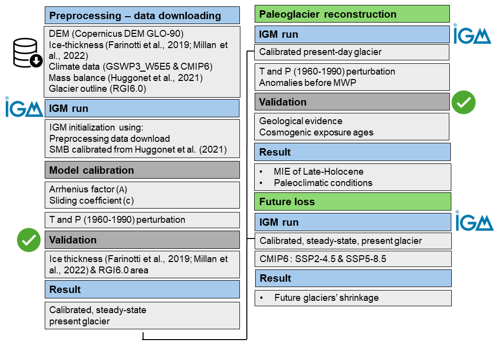
Figure 2 Flowchart followed for reconstructing past and present glaciers and projecting their future evolution based on air temperature (T) and precipitation (P). The symbols next to the graph are included to make it easier to visually associate elements and to enhance interpretability within the figure.

5 Results

5.1 IGM parametrization and calibration

For most IGM parameterizations, glacier growth occurred until 350 to 600 years of spin-up. The latest year of the spin-up simulation is subsequently validated against ice thickness estimates (Farinotti et al., 2019; Millan et al., 2022). The error metric values for ice thickness and area resulting from the IGM calibration and parametrization process are shown in Figs. 3, 5, S1, and S2. Using a calibrated melt rate factor, the most favorable range for achieving accurate results for present-day data is a perturbation range of temperature from 0 to −0.5 °C with respect to the baseline climate (Figs. 3 to 5). The largest errors in ice thickness and glacier area were observed for the A=34 MPa⁻³ a⁻¹ and c=0.01 km MPa⁻³ a⁻¹ IGM configuration. This configuration tended to overestimate ice thickness for both global-scale ice thickness references (Figs. 4 and 5). Additionally, using the default configuration and reducing the temperature to $<-\mathrm{0.5}$ °C over the baseline climate led to overestimations of ice thickness.

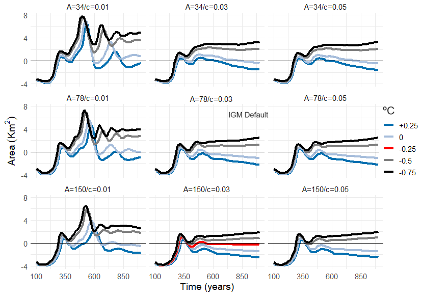
Figure 3 Difference compared to the RGI6.0 area and IGM outputs within a 1000-year spin-up. Data are grouped by changes in temperature (colors) and in A and c options (boxes). The selected configuration (A=150 MPa⁻³ a⁻¹ and c=0.03 km MPa⁻³ a⁻¹, −0.25 °C with respect to the baseline climate) is shown in red.

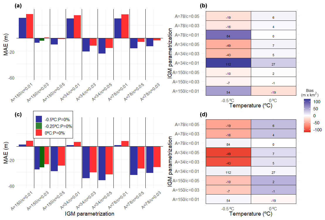
Figure 4 Ice thickness MAE between Farinotti et al. (2019) and IGM outputs after spin-up with different A and c parameterizations and perturbations of temperature (a). The selected configuration is shown in green. Ice thickness MAE values from (a) multiplied by the difference between the RGI6.0 area and the IGM outputs (bias) for different A and c parameterizations and perturbations of temperature (b). Panels (c) and (d) are the same as (a) and (b), respectively, but for ice thickness estimates from Millan et al. (2022).

Trial-and-error parameterizations of A and c revealed that optimal results were achieved for A=150 MPa⁻³ a⁻¹ and c=0.03 km MPa⁻³ a⁻¹. These outputs of the IGM align with those of Farinotti et al. (2019). However, both the IGM and Farinotti et al. (2019) overestimate ice thickness compared to Millan et al. (2022) (Figs. 4 and 5). Setting A=150 MPa⁻³ a⁻¹ and c=0.03 km MPa⁻³ a⁻¹, with a slight variation in terms of temperature (−0.25 °C) over the baseline climate, resulted in very similar accumulated ice thickness to Farinotti et al. (2019) (MAE of 4 m; Fig. 4a), a minimal RGI6.0 area bias (Figs. 3 and 4b), and very-stable-state glacier conditions for >500 years (Fig. 3). This configuration also minimized errors compared to the Millan et al. (2022) dataset (MAE of 24 m) (Fig. 4c). Glacier reconstruction and projection are based on this parametrization option. Additionally, the default IGM configuration (A=78 MPa⁻³ a⁻¹ and c=0.03 km MPa⁻³ a⁻¹), with the temperature perturbation that results in the lowest error, is included in past and future simulations to account for uncertainties in ice flow dynamics. Past reconstructions and future glaciated-area simulations are performed using the calibrated melt rate, as well as low (3) and high (9) melt rates, which define the confidence intervals for past and future projections. These melt rates are calibrated to reproduce present-day conditions. To achieve this, temperature adjustments relative to the baseline climate were set to +1.25 °C for the low melt rate and −1.5 °C for the high melt rate (Figs. S1 and S2).

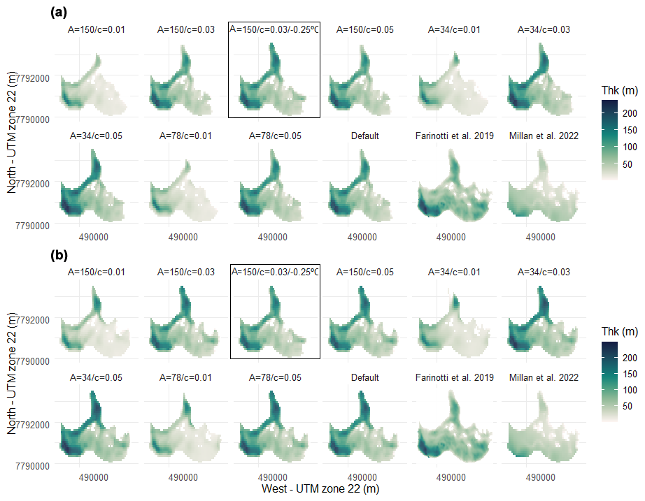
Figure 5 Average ice thickness data from Farinotti et al. (2019) and Millan et al. (2022), along with examples of IGM configuration options using different A and c parameters for the selected configuration (highlighted with a black square), are shown for a temperature of 0 °C with respect to the baseline climate (a) and a temperature of −0.5 °C with respect to the baseline climate (b). The ice thickness values of the IGM shown are the result of steady-state glacier conditions.

5.2 Late Holocene maximum glacier extension and paleoclimatic conditions

The temperature evolution from the LGM to 2000 CE, as reconstructed from GrIS ice cores and Greenland margins (Buizert et al., 2018), is shown in Fig. 6. The Camp Century and Disko Bay–Jakobshavn ice cores exhibit similar temperature trends compared to the baseline climate period, although they display larger temperature anomalies, with the warmest conditions being recorded during the Holocene Warm Period (HWP; ∼9–5 kyr ago) (up to 3 °C with respect to the baseline climate period). A long-term cooling trend is detected for the Late Holocene, with moderate anomalies and high yearly oscillations of around ±1 °C between the Dark Ages Cold Period (∼400 to 765 CE; Helama et al., 2017) and the MWP for Disko Bay–Jakobshavn (Fig. 6). However, colder temperatures are found in the Camp Century ice core. For both locations, the coldest temperature anomalies of ca. −2 °C compared to the baseline climate are found during the LIA.

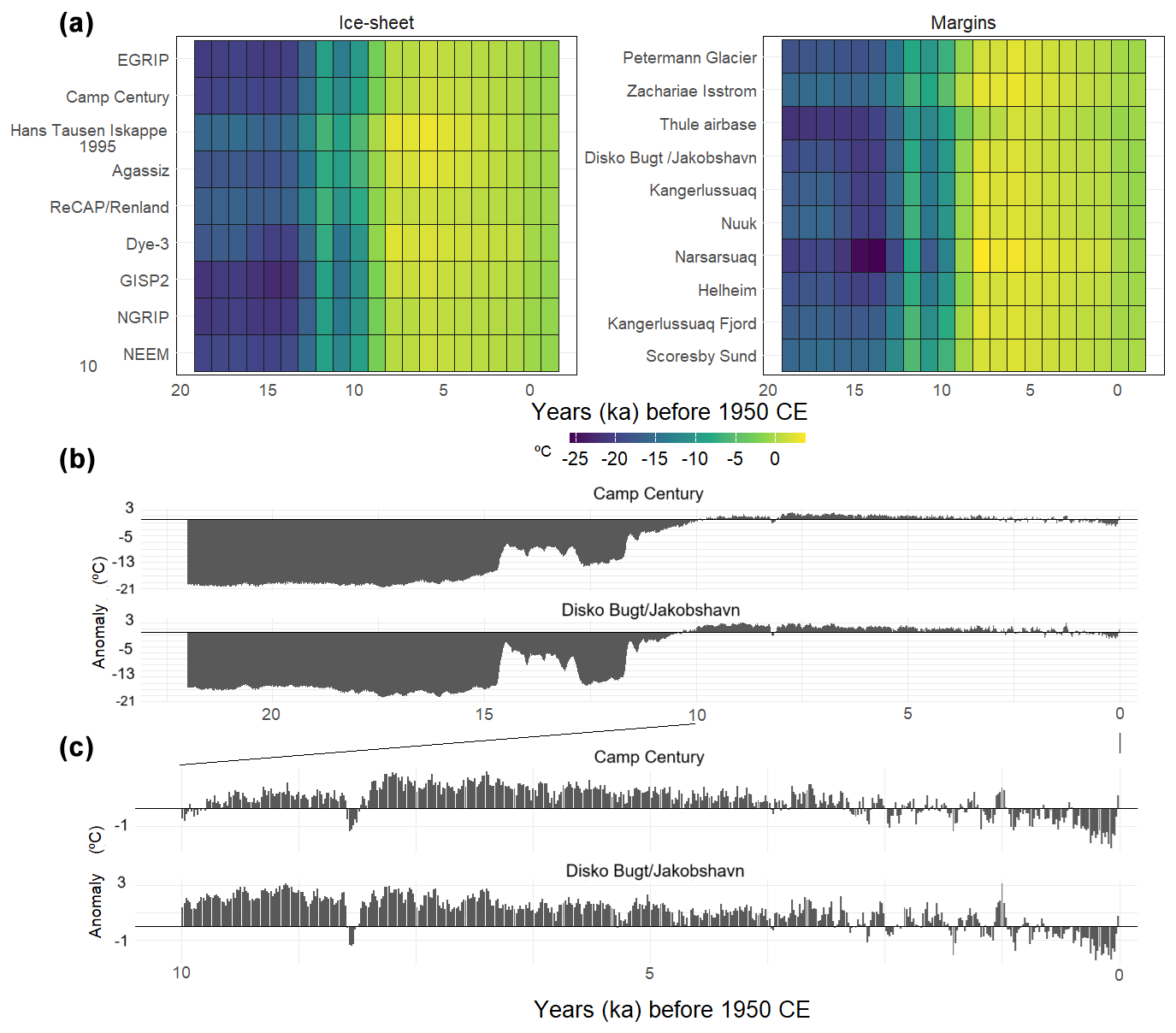
Figure 6 Air temperature anomalies from the LGM period to the present reconstructed from ice core records of the GrIS and Greenland margins (a). Air temperature anomalies from the ice cores near to the glacier reconstructed in central western Greenland (Camp Century and Disko Bay–Jakobshavn) (b). The black squares highlighted in (a) correspond to the specific locations shown in (b). Air temperature anomalies from 10 ka to 1950 (c). Air temperature anomalies are calculated based on the difference between the average annual air temperature from the baseline climate (1960–1990 period) and the annual air temperature for each location. Data were obtained from the reconstruction available from Buizert et al. (2018).

Future CMIP6 SSP2–4.5 and SSP5–8.5 anomalies with respect to the baseline climate are shown in Fig. 7. The temporal evolution of temperature follows a similar warming rate for both scenarios until 2040, after which there is an acceleration of warming for SSP5–8.5. The increase in temperature relative to the baseline climate for SSP2–4.5 is 3.1 °C by 2050 and 4.2 °C by 2100, whereas, for SSP5–8.5, it is 3.4 °C by 2050 and 6.1 °C by 2100. Thus, CMIP6 (SSP2–4.5 and SSP5–8.5) anomalies with respect to the baseline climate are similar to HWP for 2050 but higher by a factor of 3 for SSP5–8.5 by 2100 (Fig. 6). Precipitation also shows an increase with respect to the baseline climate, which is more pronounced for SSP5–8.5 towards the end of the 21st century. SSP2–4.5 precipitation anomalies with respect to the baseline climate are +20 % by 2050, increasing to +26 % by 2100. For SSP5–8.5, precipitation increases by +20 % by 2050 and +38 % by 2100.

For the 2050–2060 period, summer temperatures are projected to range from 2 °C under SSP2–4.5 to 3 °C under SSP5–8.5. For the 2090–2100 period, winter temperatures are projected to range from 5 °C under SSP2–4.5 to 8 °C under SSP5–8.5 (Fig. S3). Regarding snowfall, for the 2050–2060 period, SSP2–4.5 and SSP5–8.5 project anomalies of 12 % and 16 %, respectively (Figs. S4 and S5). For the 2090–2100 period, anomalies with respect to the baseline climate are 18 % and 22 % for SSP2–4.5 and SSP5–8.5, respectively. Other months show decreases in snowfall, except for spring, which shows a 3 % increase for both the SSP5–8.5 and SSP2–4.5 scenarios for the 2050–2060 and 2090–2100 periods.

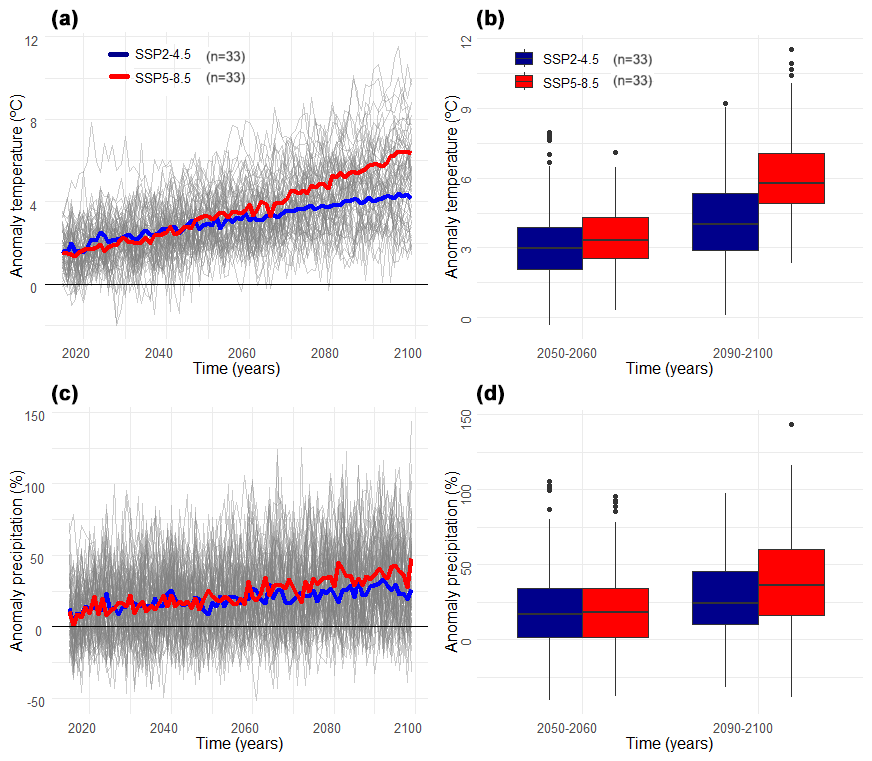
Figure 7 Temporal evolution of CMIP6 SSP2–4.5 and SSP5–8.5 temperature anomalies with respect to the baseline climate period (a). Comparison of CMIP6 SSP2–4.5 and SSP5–8.5 temperature anomalies with respect to the baseline climate period for the 2050–2060 and 2090–2100 temporal periods (b). Panels (c) and (d) are the same as (a) and (b), respectively, but for precipitation. The dots in (b) and (d) represent the average of each CMIP6 model for the temporal period and climate variable.

We further assessed whether the temperature conditions reconstructed from ice core data are consistent with CRE dates from moraine boulders and can accurately replicate the MIE of the Late Holocene. A sensitivity analysis of temperature and precipitation was conducted. For the calibrated melt rate, temperature variations ranged from −1 to 0 °C in 0.25 °C increments. For the low-end melt rate, temperature variations ranged from 0.25 to +1.25 °C in 0.25 °C increments. Precipitation remained unchanged (0 %) or increased by 10 %. We determined the temperature and precipitation conditions that allowed the MIE of the Late Holocene glacier extension, enabling its reconstruction (Fig. 8).

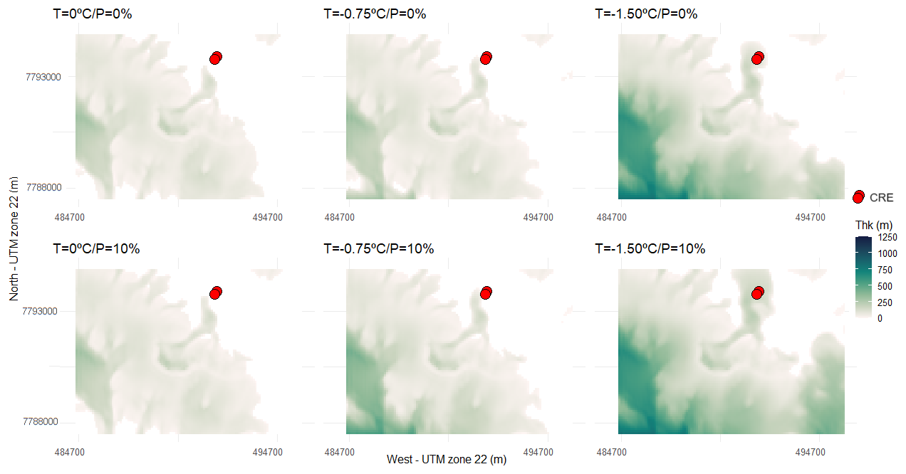
Figure 8 Location of the CRE samples (red dots) and average ice thickness (m) for various temperature (T) and precipitation (P) perturbations. The ice thickness values presented result from an initial spin-up model run, followed by a 1000-year model run to reconstruct the MIE of the Late Holocene. Data are shown for the calibrated IGM configuration and melt rate value. Reconstruction using the IGM default configuration and past reconstruction values with a low-end melt rate are shown in Figs. S6 and S7.

The assessment of past temperature and precipitation anomalies relative to the baseline climate is conducted based on the distance between the glacier tongue and available CRE dates. This analysis indicates the temperature and precipitation conditions that facilitated glacier expansion during the MIE of the Late Holocene. Note that there may be a time gap between the MIE of the Late Holocene, the timing of maximum ice expansion, and CRE ages since these ages indicate not the period of glacial growth but rather the period when moraine boulders stabilized after the formation of the moraine ridges formed by the glacier advances or stillstands. Assuming a calibrated melt rate, the minimum distance for all samples is reached when the temperature is reduced by 1 °C, while precipitation remains unchanged. Similarly, a 0.75 °C temperature reduction combined with a 10 % increase in precipitation relative to the baseline climate also leads to glacier advances reaching the limit marked by the dated moraine boulders (Figs. 8 and 9). These findings suggest that temperature anomalies leading to glacier extension up to the MIE of the Late Holocene ranged from, at least, temperatures of −0.75 °C and precipitation of +10 % to temperatures of $\le -\mathrm{1}$ °C and precipitation of 0 % relative to the baseline climate (Fig. 9). However, a variation in precipitation of 10 % is unlikely according to paleoclimate reconstructions for the Late Holocene (Badgeley et al., 2020). This suggests that using a calibrated melt rate factor with a temperature between 0.75 and 1 °C from the baseline climate and with no changes in precipitation is the most plausible climate scenario.

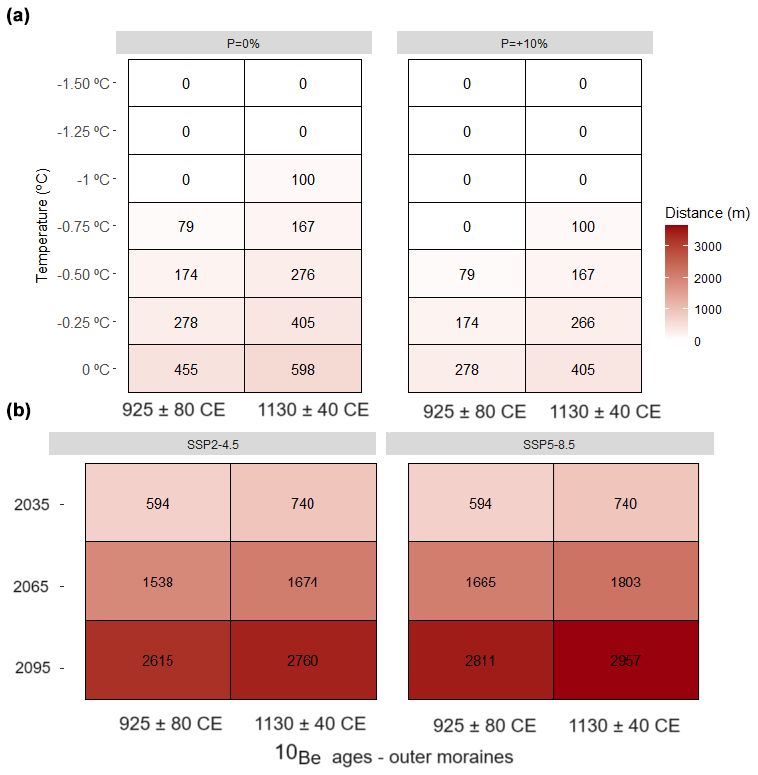
Figure 9 Differences in pixel distance (m) between the nearest modeled glacier extension and the sample age location (x axis) across various air temperature (y axis) and precipitation options (boxes) (a) using a calibrated melt rate. Differences in pixel distance (m) between the nearest modeled glacier extension and the sample age location (x axis) and projected glacier shrinkage for CMIP6 scenarios (boxes) and different years (y axis) (b).

Despite the model being calibrated and validated with three independent sources (Figs. 2–5), an uncertainty estimation of ice thickness and glaciated-area changes was performed. This estimation was based on variations in the melt rate, the ice dynamics IGM configuration, and the temperature lapse rate (Figs. S6–S9). The highest uncertainty (5 %) is attributed to the melt rate factor. The glaciated area and ice thickness decreased by 15±5 % (Fig. 10) compared to the glacier-covered surface during the MIE of the Late Holocene, where the standard deviation (±) accounts for the influence of the calibrated (−20.1 % ice thickness anomaly) and low-end melt rate factors (15.2 % ice thickness anomaly). A detailed secondary analysis was conducted by comparing the calibrated and default IGM configurations. The calibrated IGM configuration, along with the default A and c parameters, results in minor changes (<4 %) in ice thickness anomalies while maintaining the same temperature offsets (Figs. S6 and S7). Furthermore, a sensitivity analysis of the temperature lapse rate before bias correction shows small variations in ice thickness anomalies relative to the present day. A lower lapse rate (−0.55 °C m⁻¹), the applied lapse rate (−0.65 °C m⁻¹), and a higher lapse rate (−0.75 °C m⁻¹) result in a 3 % difference in ice thickness anomaly (Fig. S8).

5.3 Future glacier changes

Assuming a calibrated melt rate factor, the future climate for 2060 leads to a glacier tongue recession ranging from 1674 m (SSP2–4.5) to 1903 m (SSP5–8.5) relative to the MIE of the Late Holocene (Figs. 9 to 11). By 2090, glacier reduction is projected to reach up to 2760 m (SSP2–4.5) or 2957 m (SSP5–8.5). The rate of ice loss from the MIE of the Late Holocene to the present (15±5 %) will more than double (40±9 %) after the 2030–2040 period (Fig. 10), regardless of the CMIP6 scenario, with the standard deviation (±) reflecting the influence of the melt rate factor. By 2070–2080, ice loss will accelerate further, reaching anomalies of $-\mathrm{56}\pm \mathrm{6}$ % (SSP5-8.5). By 2100, under SSP5–8.5, ice thickness will decline to a maximum loss, leading to the disappearance of the glaciated area (Figs. 11, S10, and S11).

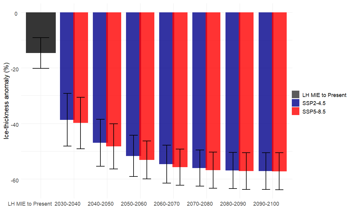
Figure 10 Ice thickness anomalies with respect to present-day glaciated area for the MIE of the Late Holocene (LH) and future CMIP6 SSP2–4.5 and SSP5–8.5 scenarios. The anomaly in ice thickness is calculated by taking the difference between the MIE of the Late Holocene and future ice loss changes and the present-day accumulated yearly ice thickness. This difference is then divided by the present-day accumulated yearly ice thickness and multiplied by 100. The column bars represent the mean ice thickness anomalies, whereas the error bars represent the standard deviation of the anomalies, which reflect the variability associated with the different melt rate factors.

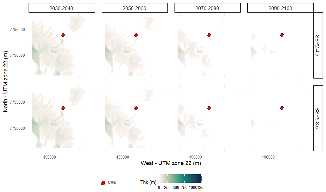
Figure 11 Location of the CRE samples (red dots) and average ice thickness (m) for future CMIP6 SSP2–4.5 and SSP5–8.5 scenarios and different temporal periods. The ice thickness values shown are the result of performing a spin-up model run reaching steady-state conditions and subsequently performing a model run with CMIP6 projections from the present day to 2100. Data are shown for the calibrated IGM configuration and melt rate values. Future simulations using the IGM default configuration and a high-end melt rate are shown in Figs. S10 and S11.

6 Discussion

6.1 Glacier modeling as a tool to understand paleoclimate conditions

The range of temperature decreases (0.75 to 1 °C) that obtained the best results in terms of reproducing glacier MIE of the Late Holocene is consistent with past temperature anomalies in western and southern Greenland found in previous works. In particular, this range of temperature anomalies falls within estimates of ∼1.5 °C cooler temperature at 1850 CE with respect to the 1990s (Dahl-Jensen et al., 1998). In southern western Greenland, temperature estimates derived from geospatial reconstructions of ELAs that attributed historical MIE to the LIA suggest temperatures ranging from around −0.4 to −0.9 °C (Larocca et al., 2020). Employing a similar methodology, other studies have found temperature anomalies during the LIA to be $-\mathrm{1.1}\pm \mathrm{0.6}$ °C, with no observed changes in precipitation (Brooks et al., 2022).

However, the MIE of the Late Holocene in central western Greenland, defined by the most recent moraine complexes, suggests an earlier maximum glacier extent than in other areas in the Northern Hemisphere when the LIA glacier expansion was much more extensive (Young et al., 2015). In this sense, the temperature indicated within the northern-hemispheric-scale reanalysis for the MWP is not consistent with the MIE obtained from glacier moraines dated with CRE in western Greenland (Jomelli et al., 2016; Biette et al., 2018). Indeed, Biette et al. (2018) modeled the outlet glacier of the Lyngmarksbræen ice cap (Disko Island) and tested its sensitivity to temperature and precipitation using a PDD approach guided by temperature anomalies from a lake sediment located 250 km south of Disko Island (D'andrea et al., 2011). They demonstrated that the MIE of the Late Holocene during the late MWP (1200±130 CE) occurred when temperatures ranged from −1.3 to −1.6 °C and that precipitation changed by ±10 % (Biette et al., 2018). Considering the fact that the baseline climate period of our work is 1960 to 1990 and that anomalies are considered up to the end of the 20th century, our results are similar to these reported temperature and precipitation values. These results are in line with a decrease in summer temperature from −0.5 to −3 °C at around 250 km from Disko Island during the MWP, as obtained from lacustrine (alkenone-based lake sediment) reconstructions, and a second cold phase during the LIA (D'andrea et al., 2011). These cold conditions have been linked to multi-decadal cold spells intense enough to cause a major advance of Baffin Bay during the MWP (Young et al., 2015; Jomelli et al., 2016). These glacier advances were also observed in other Northern Hemisphere glaciers and may also have been enhanced by volcanic eruptions (Solomina et al., 2016). The reconstructed glacier advances were probably linked with a recurrent positive NAO in western Greenland and at Baffin Bay during the MWP that lead to cool conditions (Young et al., 2015). However, other studies suggested that the NAO was not predominantly positive during this period (Lasher and Axford, 2019). There are also studies suggesting cold sea surface temperatures observed during the MWP (Sha et al., 2017), while others suggest warmer conditions during the MWP compared to during the LIA (Perner et al., 2011).

The MIE of the glaciers in the study area was reached during the MWP (1130±40 CE and 925±80 CE) (Young et al., 2015), which has been suggested to be linked to increased snowfall rates that counterbalanced the glacier ablation mass losses during the MWP, which were slightly higher than those during the LIA (Osman et al., 2021). However, an increase in precipitation of +10 % with respect to the baseline climate period is not able to counterbalance glacier recession under a change of $<-\mathrm{0.5}$ °C with respect to the baseline climate (Fig. 9). The sensitivity analysis performed here reveals that the glaciated area did not experience isothermal conditions within the 1960–1990 period, and a small decadal variation in temperature with respect to the baseline analysis of temperature and precipitation performed in this work is consistent with previous works that suggest a variation of around 90 % and that glacier maximum extension dynamics are linked with summer temperature (Miller et al., 2012; Young et al., 2015).

6.2 Central western Greenland ice loss and comparison with other Greenland areas

The reconstructed MIE of the Late Holocene represents the phase with the most recent widespread glacier advances from Nuussuaq Peninsula, which occurred prior to the LIA (Schweinsberg et al., 2017, 2019). The maximum glacier advance reconstructed in this work for central western Greenland is not consistent across Greenland. The northern GrIS exhibits stability during the Late Holocene, with advances at 2.8 ka and 1650 CE (Reusche et al., 2018). In particular, the lengths of northwestern glaciers were similar from 5.8 ka until the onset of the LIA (Søndergaard et al., 2020). In the Bregne Ice Cap (eastern Greenland), glacier length dating reveals a peak during the LIA (∼0.74 ka; Levy et al., 2014). However, in the Renland Ice Cap (eastern Greenland), glaciers exceeded present limits at 3.3 ka and around 1 ka, which is similar to LIA glacier advance (Medford et al., 2021). In central eastern Greenland, cold climate conditions occurred during the LIA at the Stauning Alps, with a peak at 0.78±0.31 ka (Kelly et al., 2008), and at the Istorvet Ice Cap, which reached its maximum Holocene extent at 0.8±0.3 ka (Lowell et al., 2013). This expansion observed in eastern Greenland corresponds with peak glacier extensions seen in Iceland, attributed to the LIA (Flowers et al., 2008). Different asymmetries between Greenland sectors are seen historically, as revealed by long-term GIC recession, which is larger in western Greenland than in the east, which has been attributed to the positive oscillation of the NAO since the LIA that led to warmer conditions in western Greenland due to the west–east NAO dipole (Bjørk et al., 2018).

In central western Greenland, most of the studies focusing on Late Holocene glacial history come from near Disko Island (Ingolfsson et al., 1990; Humlum, 1998; Yde and Knudsen, 2007; Citterio et al., 2009; Jomelli et al., 2016). In the eastern fringe of Greenland, the ELA from the LIA is estimated to be ca. 550±500 m, contrasting with values of 200–300 m seen elsewhere in the island (Ingolfsson et al., 1990). In the western section, however, the ELA during the LIA was estimated to be 450±420 m (Humlum, 1998). As in Nuussuaq Peninsula, the Holocene maximum extension in Disko Island is evidenced by moraine systems exhibiting a fresh, partly unvegetated appearance, with a prevalence of Rhizocarpon geographicum in these moraines (Humlum, 1987). This absence of Holocene moraine systems beyond the LIA moraines indicates that the advance of the LIA represents the maximum extension of this glacier since the Late Holocene (Humlum, 1999). This moraine evidence has been used to estimate the ELA (Brooks et al., 2022; Carrivick et al., 2023). In particular, using geospatial methods, Carrivick et al. (2023) attributed this trimline to the maximum extent of the LIA and concluded that Greenland GICs lost 499 Gt from the end of the LIA, corresponding to a sea level equivalent of 1.38 mm. Similarly, in southern western Greenland, 42 GICs lost 48 % of their area between the LIA and 2019 (Brooks et al., 2022). These values are higher than the 15±5 % ice thickness reduction from the MIE of the Late Holocene with respect to the present-day glaciated area reported in this work. The differences could be attributed to the local relief configuration, as well as to the northern aspect of the reconstructed glacier area and methodological variances. Additionally, while we are employing a glacier modeling approach constrained by geological records of a specific age, previous studies have estimated distances based on ELAs and geospatial methods that account for spatial distances between present-day glacier tongues and maximum historical moraines that could have been formed prior to the LIA. According to remote sensing data, in Disko Island, GIC inventories and monitoring from 1953 to 2005 indicate that the average recession during this time frame amounted to 11 % of the glacier lengths recorded in 1953 (number of glaciers, n=172) and 38 % of the distance between LIA moraines and glacier termini in 1953 (n=87) (Yde and Knudsen, 2007). These values are lower than those observed at Pjetursson Glacier (Disko Island), which has retreated since the LIA, with a decrease in total glacier area of around 40 % by the end of the 20th century according to geospatial methods (Bøcker, 1996). Using remote sensing data, the glacier shrinkage from the LIA until 2001 in central western Greenland was estimated, showing a reduction of ∼20 % of the area (Citterio et al., 2009).

Currently, the modeled glaciated area and volume are out of balance with respect to the temperature from 1990 to present (figure not shown), necessitating the simulation of the glaciated area using temperature and precipitation data from the 1960–1990 period (Fig. 2). This indicates a committed ice loss regardless of future climate scenarios. Future projections show a remarkable increase in temperature, reaching HWP anomalies by 2050 and tripling HWP anomalies by 2100 under SSP5–8.5. Our results indicate that glacier mass loss by >2070 will double the ice loss from the MIE of the Late Holocene to the present. Precipitation is projected to increase by 20 % (2050; SSP2–4.5 and SSP5–8.5) up to 38 % (2100; SSP5–8.5) compared to the baseline climate but cannot counterbalance glacier losses, and the modeled glaciated area is expected to disappear by 2090–2100 (Fig. 11). The data presented in this work suggest that future glacier ice loss will occur at unprecedented rates compared to the period of the MIE of the Late Holocene to the present.

According to CMIP6 projections for the near-ice-free zones of Disko Island, this temperature increase is explained by increases in longwave radiation and slight variations or decreases in shortwave radiation (Bonsoms et al., 2024a). Future winter temperatures are expected to remain below isothermal conditions, leading to more snowfall during winter (i.e., +22 % for SSP5–8.5 for the 2090–2100 period relative to the baseline climate). The increase in snowfall, however, cannot counterbalance glacier shrinkage, and a 10 % increase in precipitation has minimal impact on glacier area and thickness variability (Fig. 8). Snowpack projections for a near-ice-free region of Disko Island align with these findings, indicating decreases in snow depth and snowfall fraction, along with increases in snow ablation (Bonsoms et al., 2024a). For the GrIS, previous studies projected a larger SMB decrease in ice sheet margins due to higher melting and lower accumulation compared to the GrIS interior, pointing out that increases in snowfall are insufficient to counterbalance the increased runoff (Fettweis et al., 2013). Yet, CMIP6 models are unable to capture the increase in anticyclonic events in Greenland since the 1990s (Delhasse et al., 2021), which has driven increased melting and extreme melting events in the GrIS (Bonsoms et al., 2024b).

Greenland GIC numerical modeling reconstructions are scarce in comparison with GrIS numerical modeling works, including paleoclimate modeling (Huybrechts, 2002), model parameter sensitivity studies (Cuzzone et al., 2019), or GrIS Holocene evolution reconstructions constrained with geological records (i.e., Simpson et al., 2009; Lecavalier et al., 2014, Briner et al., 2020). GICs make a modest (11 %) contribution to total Greenland ice loss but exhibit a fast response to warming (Khan et al., 2022). While we modeled the response of a glaciated area in eastern Nuussuaq, future studies should compare these ice loss rates with GrIS trends, which exhibit a slower response to warming (Ingolfsson et al., 1990). The anticipated glacier retreat has important environmental implications, including increased freshwater release into the North Atlantic and alterations in atmospheric and circulation patterns (Yu and Zhong, 2018), which may impact the Atlantic Meridional Overturning Circulation (Thornalley et al., 2018). Thus, Greenland glacial retreat, snow melting, and permafrost thaw will amplify the release of greenhouse gases and potentially trigger major consequences at the global scale (Miner et al., 2022). Negative mass balances will change geomorphological and permafrost patterns (Christiansen et al., 2010) and ecosystem dynamics in ice-free zones by modifying maritime (Saros et al., 2019) and terrestrial phenological and fauna distributions (John Anderson et al., 2017).

6.3 Atmospheric forcing and numerical modeling considerations

This work is based on the GSWP3 W5E5v2.0 climate dataset, which is based on ERA5 reanalysis data bias-adjusted over land (Lange et al., 2021). ERA5 incorporates observations via a data assimilation system combining observations, modeling, and satellite data and was previously validated in Greenland (Delhasse et al., 2020). ERA5 has been used to force state-of-the-art regional climate models, showing good agreement with observations (Box et al., 2022). Our results are consistent with previous works that provided a glacier reconstruction based on outputs of MAR forced with ERA5 and a PDD model in Disko Island (central western Greenland) (Biette et al., 2018). Indeed, results are similar to geospatial reconstructions in other Greenland sectors (i.e., Brooks et al., 2022). The main conclusions of this work are consistent with paleo GrIS reconstructions and projections in the central western GrIS (Briner et al. 2020).

A more sophisticated glacier modeling experiment will require data from coupled regional circulation models, which account for changes in large-scale circulation. However, glacier modeling driven by paleoclimate simulations has uncertainties and large variability between models as previous works in the study area have shown that paleoclimate simulations cannot reconstruct Late Holocene glacier dynamics in the study area (Jomelli et al., 2016; Biette et al., 2018). In this work, a sensitivity analysis of precipitation and temperature is conducted to reconstruct glacier MIE based on cosmogenic data, and, therefore, results are analyzed based on anomalies with respect to a baseline climate (1960–1990), which is sufficiently long to consider climate interannual variability and is marginally affected by climate warming.

The IGM has been previously validated for modeling the present and projecting the future evolution of alpine glaciers, providing reliable results (Cook et al., 2023, and references therein). Here, we have performed an IGM parameter tuning to accurately simulate present-day glacier conditions. We cross-validated results against two independent ice thickness products (Farinotti et al., 2019; Millan et al., 2022) and RGI6.0 observations. The data show good agreement when compared to Farinotti et al. (2019) but lesser agreement when compared to Millan et al. (2022) (Fig. 4). These differences could be attributed to the different glacier methodologies: Farinotti et al. (2019) based their work on an ensemble of five glacier models founded on ice flow physics, whereas Millan et al. (2022) based their work on glacier flow mapping. Further research should analyze these differences. As with most numerical modeling experiments, past and future ice flow parameters are likely to be different from present-day parameters due to unknown variables such as variations in basal conditions, bedrock topography, and ice rheology. This issue was minimized by analyzing glacier simulations using both the IGM default configuration and a calibrated IGM option, validated against available mass balance data, observations, and ice thickness products. This approach allowed for isolating and better analyzing the effects of temperature and precipitation on past and future glacier trends.

As with most paleo glacier models, the IGM relies on a PDD approach, which is an approximation that does not account for the surface energy balance (SEB) driving melting. However, the SEB components required for glacier modeling are uncertain for the spatial and temporal scales analyzed in this study. The PDD approach is based on a temperature index model. Impurities on the ice (such as algae and dust) are not directly considered but indirectly inferred by the melt rate factor. The IGM configuration for the calibration and correction process of precipitation and temperature is based on OGGM v1.6.1 (Maussion et al., 2019; Schuster et al., 2023). This calibration corrects precipitation and temperature to match the geodetic mass balance at the glacier level (Hugonnet et al., 2021). This product was selected due to the lack of long-term past and present in situ mass balance measurements in the study area. The errors of Hugonnet et al. (2021) product therefore influence the glacier modeling results when using the calibrated melt rate factor. The OGGM v1.6.1 calibration of bias correction has recently been compared and cross-validated for glacier modeling of past and future glacier projections, demonstrating reliable results (i.e., Aguayo et al., 2023; Zekollari et al., 2024, and references therein). Additionally, we addressed uncertainties in temperature lapse rates and PDD calibration by incorporating both low-end and high-end melt rate factors, providing a confidence interval for past and future simulations.

7 Conclusions

This study provides a long-term perspective on the dynamics of GICs in eastern Nuussuaq, central western Greenland, in response to climate change. By integrating geological records, ice thickness estimates, and climate model projections, we contextualize present and future glacier loss within the Late Holocene.

The IGM was calibrated and validated using various parameterizations to accurately simulate glacier ice thickness and area. After a long-term spin-up simulation, the model stabilized, closely matching available ice thickness data and satellite observations from RGI6.0. The optimal configuration reproduced ice thickness estimates with an error of less than 10 % of the total accumulated ice thickness for the modeled area. Subsequently, the model was forced with different temperature and precipitation scenarios, validated with CRE records, enabling the quantification of glacier retreat since the MIE of the Late Holocene. For future projections, the IGM was driven by CMIP6 climate scenarios (SSP2–4.5 and SSP5–8.5), providing a comparative framework for past and future glacier recession in a changing climate. The main conclusions of this study are as follows:

• The MIE of the Late Holocene was reached when temperatures were 0.75 to 1 °C lower than the baseline climate period (1960–1990) under a calibrated melt rate factor.

• Currently, glaciated-area ice thickness has retreated by 15 % (low-end melt rate) to 20 % (calibrated melt rate) compared to the MIE of the Late Holocene.

• Glacier mass loss is projected to occur at an unprecedented rate within the Late Holocene. Future simulations for 2070–2080 indicate a retreat that is more than double ($-\mathrm{56}\pm \mathrm{6}$ %) the ice loss from the MIE of the Late Holocene to the present.

• The glaciated area is expected to disappear towards 2090–2100.

The results confirm the ongoing imbalance of GICs in eastern Nuussuaq, central western Greenland, and highlight the unprecedented nature of current glacier shrinkage within the Late Holocene. Projections suggest that climate change will accelerate ice loss beyond historical trends, transforming Arctic landscapes, increasing deglaciated areas, and promoting the formation of new lakes. These findings enhance our understanding of Arctic peripheral glacier responses to anthropogenic climate change, with broad implications for hydrological and ecological systems.