Anisotropic scattering in radio-echo sounding: insights from northeast Greenland

Anisotropic scattering and birefringence-induced power extinction are two distinct mechanisms affecting the azimuthal power response in radio-echo sounding (RES) of ice sheets. While birefringence is directly related to the crystal orientation fabric (COF), anisotropic scattering can, in principle, have various origins. We use curve-fitting techniques to evaluate the relative contributions of anisotropic scattering and birefringence in quad-polarized ground-based RES measurements from the Northeast Greenland Ice Stream (NEGIS), identifying their dominance and orientation across depths of 630–2500 m. We find that anisotropic scattering clearly dominates the radar signal in most depths larger than 1200 m, while birefringence effects are most important in shallower depths and particularly in the vicinity of the ice-stream shear margins. We further find that the co-polarized power difference follows the ice-sheet stratigraphy with a notable transition in strength and/or direction at the Wisconsin–Holocene transition and in folded ice outside the ice stream, possibly indicating disrupted stratigraphy in these folded units. We conclude that small-scale fluctuations in the horizontal COF eigenvalues are the most likely mechanism responsible for the anisotropic scattering observed in our survey area. Mapping the strength and orientation of scattering in quad-polarized measurements thus has the potential to provide independent estimates of the COF orientation and distinguish ice units with different scattering properties, e.g. from different climatic periods.

1 Introduction

Radio-echo sounding (RES) is widely used for studying ice sheets, glaciers, and ice caps by sending electromagnetic waves in the radio frequency range into the ice and measuring the strength of the reflected signals as a function of time. An important observation in RES measurements is the azimuthal dependency of the return power, where the strength of the signal varies with the orientation of the polarization. This dependency is influenced by two distinct mechanisms: birefringence and anisotropic scattering (Fujita et al., 2006; Matsuoka et al., 2009). Both mechanisms can be indicative of ice properties critical to palaeoclimate and ice-dynamics research, and, while they may appear independently, they frequently coexist.

Birefringence is directly related to the preferred alignment of ice crystals, commonly known as crystal orientation fabric (COF) or lattice preferred orientation. Individual ice crystals are transversely isotropic about the crystal axis (c axis), with higher dielectric permittivity along the c axis compared to the basal plane. A systematic orientation of ice crystals in the polycrystal results in anisotropic electromagnetic and mechanical properties, along with birefringence. As electromagnetic waves propagate through ice, they decompose into two orthogonal wave components, each polarized with a principal COF axis (Hargreaves, 1977). For nadir wave propagation (the standard setup in ice-sheet RES), these polarizations lie in the horizontal plane, assuming that one eigenvector is vertical. Horizontal anisotropy causes wave speed differences for these two wave components, which leads to travel-time differences of reflected signals for radar polarization parallel and perpendicular to COF axes (Gerber et al., 2021; Zeising et al., 2023). This effect can also manifest as double reflections in radargrams that are misaligned with the COF (Nymand et al., 2025). Additionally, interference between the two waves leads to power extinction nodes when the phases are shifted by half a wavelength upon reception (Fujita et al., 2006). In radargrams, these appear with a vertical spacing that depends on the strength of horizontal anisotropy and radar frequency (Young et al., 2021; Gerber et al., 2023) and with an azimuthal periodicity of 90° in both co-polarized (transmit and receive polarizations are parallel) and cross-polarized (transmit and receive polarizations are perpendicular) measurements. In the absence of anisotropic scattering, co-polarized power extinction (CoPE) nodes emerge at an azimuth of 45° from the principal COF axis, while cross-polarized power extinction (XPE) aligns with COF axes (see, for example, Fig. 5 in Fujita et al., 2006, for an illustrative overview). This effect persists with a 90° azimuthal periodicity, even if none of the principal directions of the COF are vertical (Rathmann et al., 2022).

Anisotropic scattering describes the directional dependence of ice's scattering properties, which causes variations in signal intensity based on the orientation of the antenna. Scattering of radio waves in ice sheets arises from two main mechanisms: volume scattering, driven by small-scale inhomogeneities within the ice, and surface scattering, caused by reflections at internal interfaces (e.g. Langley et al., 2009; Drews et al., 2012). Volume scattering includes contributions from air bubbles, dust, and impurities and shows anisotropic characteristics when these scatterers are rotationally asymmetric, such as elongated air bubbles or small-scale fluctuations in horizontal permittivities related to COF (Drews et al., 2012). Surface scattering, on the other hand, takes place at reflection horizons typically linked to volcanic eruptions and climatic transitions (Paren and Robin, 1975; Fujita et al., 1999; Hempel et al., 2000; Eisen et al., 2006); material boundaries like water, air, or sediment inclusions (Robin et al., 1969; Paren and Robin, 1975); or abrupt changes in COF (Eisen et al., 2007). Anisotropic reflections may emerge when these interfaces exhibit directional roughness (e.g. van der Veen et al., 2009; Cooper et al., 2019; Eisen et al., 2020) or involve transitions in COF with horizontal anisotropy (Eisen et al., 2007). Importantly, anisotropic scattering is distinguishable from birefringence by its azimuthal periodicity of 180° in co-polarized return power, compared to the 90° periodicity associated with birefringence (Fujita et al., 2006).

An important distinction must be made between horizontally anisotropic COFs causing birefringence and COFs that lead to anisotropic scattering. Horizontally anisotropic COFs are characterized by a large difference in their horizontal eigenvalues, causing strongly birefringent properties, and are typically found in dynamic areas of ice sheets. Examples of COFs with strong horizontal anisotropy include vertical girdles often found in flank flow (e.g. Fitzpatrick et al., 2014; Stoll et al., 2024) or horizontal single maxima which develop in shear zones (e.g. Thomas et al., 2021; Gerber et al., 2023). The scattering property, however, seems to arise from variations in the directional relative permittivities (i.e. ${\mathit{\epsilon }}_x^{\prime }$, ${\mathit{\epsilon }}_y^{\prime }$) and not from the COF type itself. In other words, it is the noise of the horizontal eigenvalue distribution rather than the COF type that causes anisotropic scattering. For example, a horizontal single maximum could in theory be highly anisotropic without causing anisotropic scattering if it is perfectly constant with depth, while a weak girdle can cause stronger anisotropic scattering when the horizontal eigenvalues fluctuate with depth.

Azimuthal power fluctuations have been observed in previous airborne and ground-based polarimetric experiments, defined here as RES measurements including multiple polarization directions. Most of these studies have focused on identifying the horizontal component and orientation of electromagnetic anisotropy, typically associated with COF, and therefore relevant for ice-flow mechanics (Duval et al., 1983). This can be analysed using methods like CoPE and XPE node analysis (Young et al., 2021; Gerber et al., 2023), coherence phase analysis (Dall, 2010; Jordan et al., 2019, 2022; Ershadi et al., 2022), or travel-time differences (Gerber et al., 2023; Zeising et al., 2023). CoPE nodes, in particular, can be valuable for estimating horizontal COF anisotropy over large areas, as they can also be observed in single-polarized radar measurements (Young et al., 2021; Gerber et al., 2023), the most common type used for large-scale airborne ice-sheet surveys. However, the presence of anisotropic scattering complicates these analyses by influencing the vertical elongation and azimuthal spacing of CoPE nodes, as well as the angular width of dipole nodes in coherence phase data (Fujita et al., 2006; Ershadi et al., 2022). Therefore, understanding the role of anisotropic scattering is crucial for accurately interpreting COF anisotropy and birefringence signatures in radargrams.

In this study, we use ground-based quad-polarized (transmit and receive polarizations are sequentially rotated by 90°, resulting in two co-polarized and two cross-polarized modes) ultra-wideband RES data to quantify the relative importance of anisotropic scattering and birefringence effects in a dynamic region of the Greenland Ice Sheet (GrIS). Our study site (see Fig. 1) is located in the onset region of the Northeast Greenland Ice Stream (NEGIS), near the East Greenland Ice-core Project (EastGRIP) drill site. The NEGIS region is of particular interest due to relatively fast ice flow (reaching 55 m a⁻¹ at the drill site; Hvidberg et al., 2020) where deformation-induced anisotropic scattering mechanisms can be expected, and the COF is known to be highly anisotropic in the ice-stream centre (Stoll et al., 2024). We synthesize the full azimuthal response from quad-polarized measurements, and then we use curve-fitting methods to determine the amplitude and orientation of 90 and 180° periodic co-polarized power fluctuations at different depths, with a spacing of 5 km along the radar lines. Our results show that anisotropic scattering dominates most of the survey area, especially within the ice stream and in ice from the Wisconsin period. Additionally, the strength and orientation of anisotropic scattering correlate with ice-sheet stratigraphy, with a sharp reversal in directionality at the 11.4 ka isochrone, marking the transition from Holocene to Wisconsin ice, at a depth of approximately 1300 m outside the shear margins. We propose that small-scale vertical variations in the COF are the most probable cause of the observed anisotropic scattering patterns, making the scattering orientation a direct indicator of COF orientation.

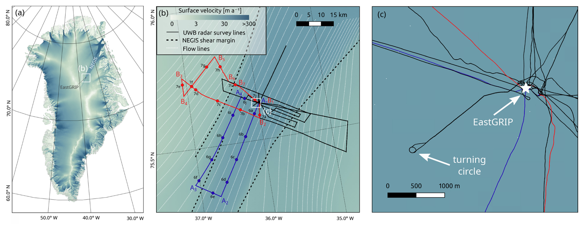
Figure 1 (a) Overview of the radar survey near the EastGRIP ice core site located in the Northeast Greenland Ice Stream (NEGIS), indicated by the enhanced surface flow velocities (Joughin et al., 2018). (b) Polarimetric RES lines are shown as black solid lines with two example radargrams (profiles A and B shown in Fig. 7) highlighted in blue and red, respectively. A₁, A₂, etc. indicate reference points of changing driving direction in Figs. 2 and 7, and dots along profiles A (6a–6j) and B (7a–7j) mark analysis points in Figs. 4 and 5. Thick dashed lines indicate the position of the shear margins, and white lines indicate the streamlines derived from surface velocities. (c) Location of the turning circle near the EastGRIP drill site. The colour scale in panel (b) also applies to (a) and (c).

2 Radio-echo sounding data and isochrone dating

The RES data used in this study were recorded in June/July 2022 with a quad-polarized ground-based system. The radar operated at a centre frequency of 330 MHz with 300 MHz bandwidth and a chirp length of 10 µs. Eight channels from the digital system were divided into 10 amplifiers with peak transmit power of 150–250 W per amplifier, feeding a 10×10 element array. This setup formed a 2.7 m×2.7 m antenna resting on a balloon and was dragged over the snow surface at an average speed of ∼3 m s⁻¹. A high-power switch coordinated the polarization of transmit and receive channels for quad-polarized recording (HH, HV, VV, and VH, where V denotes along-track polarization). The receivers were blocked during the 10 µs transmit time, corresponding to an approximate depth of 630 m for the first recorded returns. A detailed description of the radar system can be found in Yan et al. (2020).

The radar survey was conducted along the lines shown in Fig. 1, which are mostly aligned parallel/perpendicular to the general southwest to northeast surface ice-flow direction and cover a distance of approximately 450 km, spanning the entire width of the ice stream. Figure 2 shows an example radargram (profile A in Fig. 1) in the four polarization modes HH, HV, VV, and VH. Additionally, a circular radargram (turning circle) with an approximate radius of 50 m was recorded near the EastGRIP camp for testing purposes (Fig. 1c). Data processing followed a standard procedure including coherent integration, pulse compression, incoherent integration, channel integration, and interpolation to a consistent grid (Nymand et al., 2025). While synthetic aperture radar (SAR) focusing of the RES data could improve some radargram sections, challenges related to irregular tracks and high bandwidth complicated motion compensation, limiting overall improvement. Consequently, SAR focusing was not employed. The final trace spacing after processing is approximately 25–30 m on average, while it is approximately 0.7 m in the turning circle.

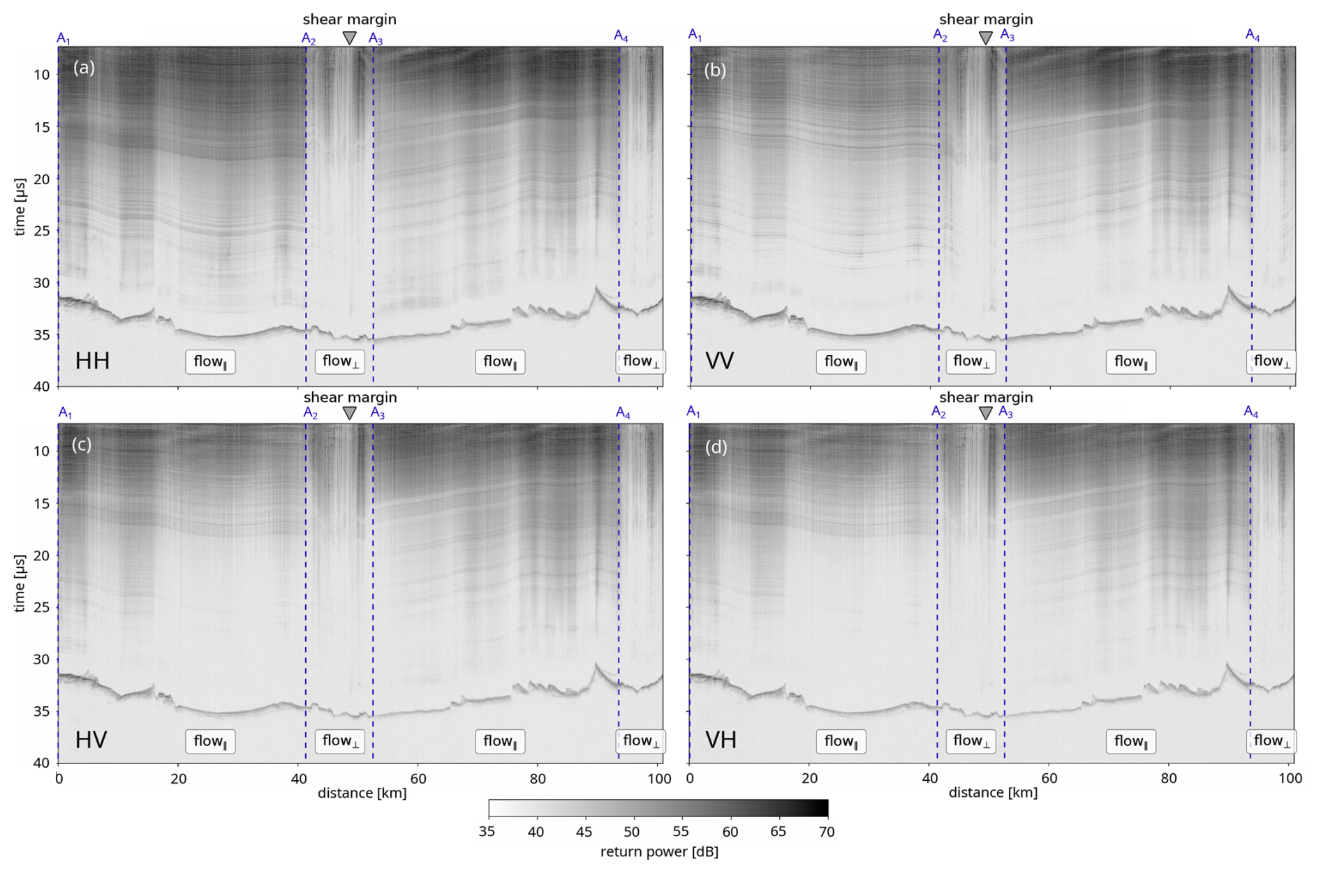
Figure 2 Example radargram (profile A in Fig. 1) recorded with the quad-polarized radar. Co-polarized profiles are shown in panel (a) (HH – cross-track) and (b) (VV – along-track). Panels (c) and (d) show cross-polarized profiles (HV and VH, where the first and last letters indicate transmit and receive polarization, respectively). Sections A₁–A₂ and A₃–A₄ are flow-parallel, while A₂–A₃ and A₄–end are flow-perpendicular.

Isochrones were traced manually for profiles A and B (Fig. 7) and dated following Gerber et al. (2021). In doing so, the travel times were converted to depth using a velocity profile inferred from the relative dielectric permittivity obtained from dielectric profiling (DEP) of the EastGRIP core (Mojtabavi et al., 2022). The DEP complex-valued, ordinary relative dielectric permittivity, ε, was measured at 250 kHz at a resolution of 5 mm, starting at a depth of 13.7 m. We used a smoothed version of the real part of the dielectric record, ε^′(z), to estimate the velocity profile in the upper 183 m by extrapolating to a surface value of ${\mathit{\epsilon }}_{\mathrm{s}}^{\prime }=\mathrm{1.55}$. Below the transition into pure ice at a depth of 183 m, we assume a constant relative permittivity in ice of ${\mathit{\epsilon }}_{\mathrm{i}}^{\prime }=\mathrm{3.15}$. The velocity profile is then obtained with

$$\begin{array}{}\text{(1)}& c\left(z\right)={\displaystyle \frac{c_{\mathrm{0}}}{\sqrt{{\mathit{\epsilon }}^{\prime }\left(z\right)}}},\end{array}$$

where ε^′(z) is the relative dielectric permittivity and c₀ is the speed of light. The age uncertainties generally increase with depth due to the timescale maximum counting error and because the existing timescale does not extend to the deepest layer traced here (see Gerber et al., 2021, for discussion of uncertainties). The deepest traced isochrone (74.7 ka; see Fig. 7) has an additional uncertainty from the layer tracing across the shear margin in profile B, particularly since the bottom part from 20 km and onward is heavily folded, causing ambiguity in matching the deepest isochrone inside and outside the shear margin.

3 Azimuthal response – model and observations at EastGRIP

The effects of anisotropic scattering and birefringence can be distinguished by their periodicity of co-polarized power anomalies, dP_HH (for definition, see Sect. S1 in the Supplement or Ershadi et al., 2022). These patterns differ because the two mechanisms are governed by distinct symmetries.

Amplitude variations due to anisotropic scattering originate from variations in scattering properties within the ice that have a two-fold symmetry. This means that the returned signal is strongest in two opposite directions, resulting in a 180° periodicity when co-polarized antennas are rotated.

In contrast, birefringence splits the transmitted radar wave into two orthogonal components that travel at different speeds through anisotropic ice. The relative amplitude of these two wave components depends on the orientation of the antennas relative to the COF axes, while the phase difference depends solely on the degree of anisotropy but is independent of the antenna orientation. Interference between the two wave components modulates the return power. A 90° rotation of co-polarized antennas flips the amplitudes of the two components, but the interference pattern remains unchanged. Therefore, birefringence creates a 90° periodicity in the co-polarized signal (Hargreaves, 1977).

Both mechanisms exhibit 90° periodicity in cross-polarized anomalies, dP_HV, because the transformation of the polarization state, whether through scattering or birefringent phase shifts, inherently alternates every quarter-wave (90°), driven by the geometry of the polarization ellipse.

The full co- and cross-polarized angular response was measured by the radar in a turning circle with approximate diameter of 50 m in the vicinity of EastGRIP (Fig. 1c). Alternatively, this response can be synthesized from a single quad-polarization measurement using the method described in Eq. (11) of Ershadi et al. (2022), which shows good agreement with the turning circle measurements (details in Sect. S2 in the Supplement). To assess the relationship between COF, birefringence, and anisotropic scattering, we compared power anomalies from a wave-propagation model (Fujita et al., 2006), which uses the COF record from the nearby EastGRIP ice core, with both the turning circle data and the synthesized azimuthal response from a single quad-polarized measurement near the turning circle. In the model, we assumed that anisotropic scattering arises solely from vertical fluctuations in horizontal eigenvalues, and birefringence is defined by the observed eigenvalue differences (Sect. S1).

To quantitatively estimate the relative importance of anisotropic scattering (180° dP_HH periodicity) and birefringence (90° dP_HH periodicity), we then fit the sum of 90°- and 180°-periodic sinusoidal signals to dP_HH as a function of azimuth θ:

$$\begin{array}{}\text{(2)}& f\left(\mathit{\theta }\right)=A_{\mathrm{180}}\sin (\mathrm{2}\mathit{\theta }+{\mathit{\phi }}_{\mathrm{180}})+A_{\mathrm{90}}\sin (\mathrm{4}\mathit{\theta }+{\mathit{\phi }}_{\mathrm{90}}).\end{array}$$

Figure 3 shows the average azimuthal co-polarized power fluctuations with the fitted function and the contributions of each component at five depth intervals. The relative importance of anisotropic scattering and birefringence is given by the fitted amplitudes A₁₈₀ and A₉₀, respectively, which are displayed on top of each panel in Fig. 3, and scattering direction is given by the fitted phases φ₁₈₀ and φ₉₀. For all three datasets, anisotropic scattering becomes increasingly important relative to birefringence with increasing depth, as the $\frac{A_{\mathrm{180}}}{A_{\mathrm{90}}}$ ratio increases for all depth increments except between panels (g) and (j). Birefringence is only dominant in shallow depths, notably in the 0–500 m interval of the model output (panel a) and the 500–1000 m interval of the turning circle (panel b). Amplitudes of anisotropic scattering are generally higher in the model compared to radar observations, possibly because the relatively low sampling rate of COF measurements with depth may fail to capture a smoother, more continuous COF-depth function as it may occur in reality.

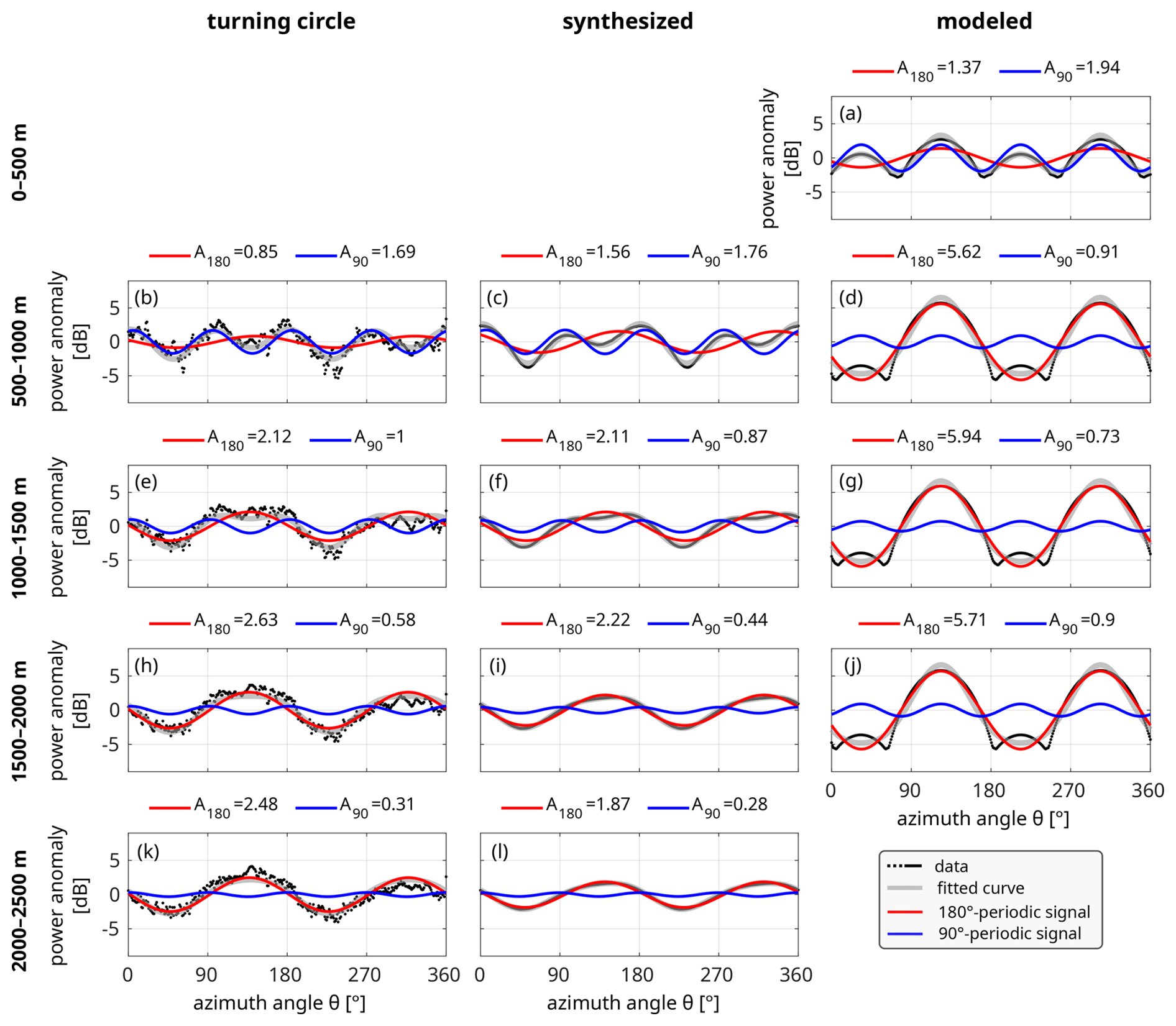
Figure 3 Depth-averaged power anomalies from turning circle (b, e, h, k), synthesized (c, f, i, l), and modelled with the COF at EastGRIP (a, d, g, j) shown in black. For all depth intervals indicated on the left side of the figure, the sum of 90° (blue) and 180° (red) periodic signals is fitted to the data points (black) using Eq. (2) and is shown in grey. The amplitudes of the corresponding 90° and 180° signals are displayed on top of each panel, indicating the relative importance of birefringence (90° periodicity) and anisotropic scattering (180° periodicity). The x axes indicate azimuth as clockwise angle from true north in all panels. The surface flow direction in this area is approximately 33° from true north (Hvidberg et al., 2020).

4 Orientation and strength of scattering and birefringence across NEGIS

We now investigate the strength and orientation of anisotropic scattering on larger spatial scales by calculating the synthesized co- and cross-polarized power anomalies and coherence phase difference at intervals of 5 km along the remaining radargrams. We use the same curve-fitting procedure as in Fig. 3 to determine the orientation and strength of anisotropic scattering and birefringence effects for different depths. The synthesized response is calculated from an average over ∼100 m distance to improve signal-to-noise level, since the driving direction at the analysis points is reasonably constant and the subsurface properties are not expected to change significantly over the corresponding distance. The curve fitting was done at every 20 m depth on the synthesized angular response averaged over a 0.2 µs interval or ∼16 m depth. Figures 4 and 5 show the co- and cross-polarized power anomalies and coherence phase, as well as the 90 and 180° amplitude–depth profile at every other analysis point (10 km spacing) for two example lines corresponding to profiles A and B in Fig. 1, respectively. The 90°- and 180°-periodic signal components of the fitted curves are displayed at 800, 1000, 1500, and 2000 m depth in the dP_HH panels. Isochrone depths, corresponding to those traced in Fig. 7, are indicated in blue in the other panels.

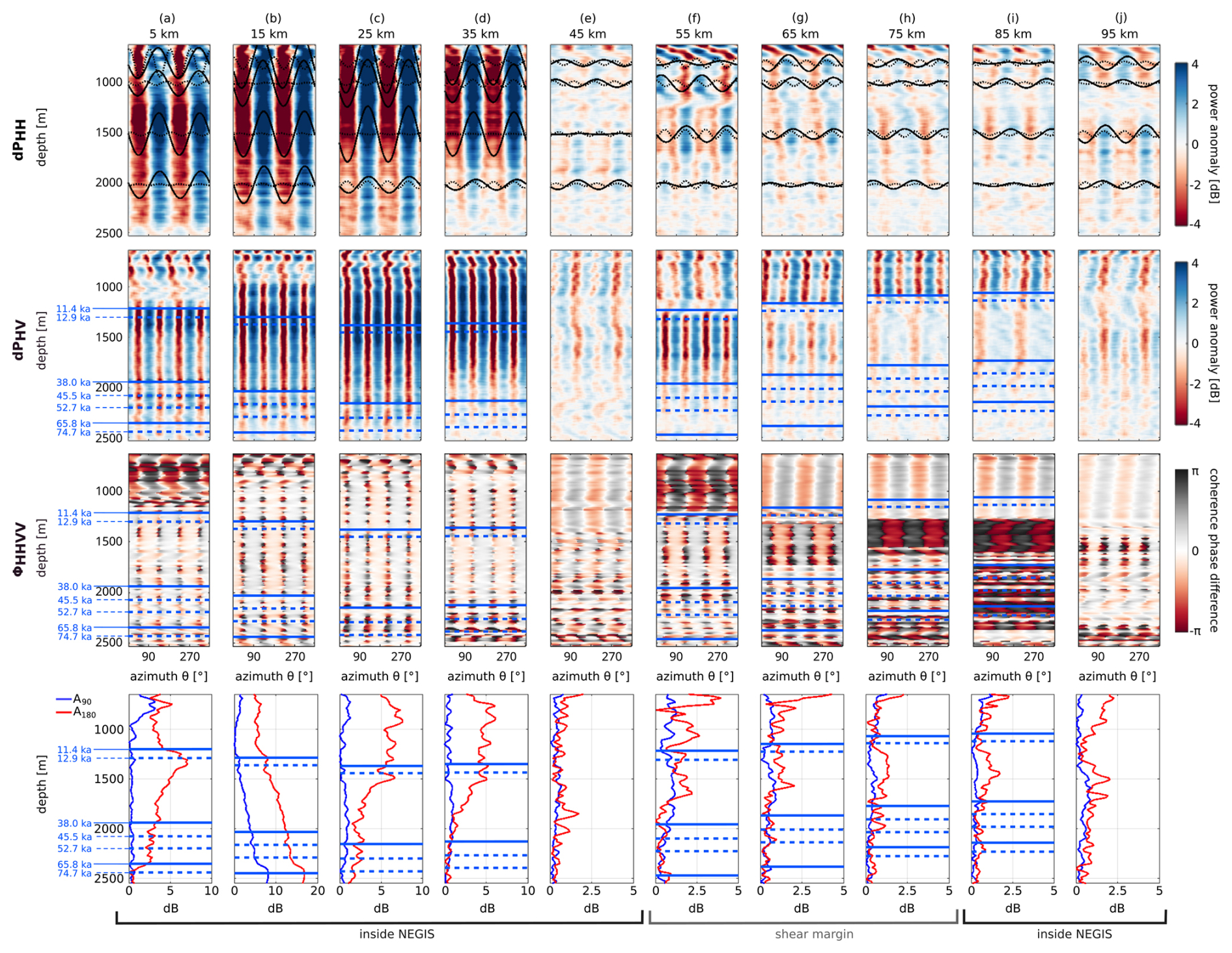
Figure 4 Synthesized azimuthal radar response for profile A: top panels show the co-polarized power anomaly dP_HH with the fitted 90°- and 180°-periodic sine curve shown as dotted and solid lines, respectively, at depths of 800, 1000, 1500, and 2000 m. Middle panels show the cross-polarized power anomaly dP_HV and coherence phase difference ϕ_HHVV. The x axis on each panel in the upper three rows shows the azimuth rotating clockwise from true north. Bottom panels show the amplitudes (in decibel) of the 90 and 180° periodic signal component with depth. Notice the different x axes of the bottom panels. Blue horizontal lines indicate the depths of isochrones traced in Fig. 7.

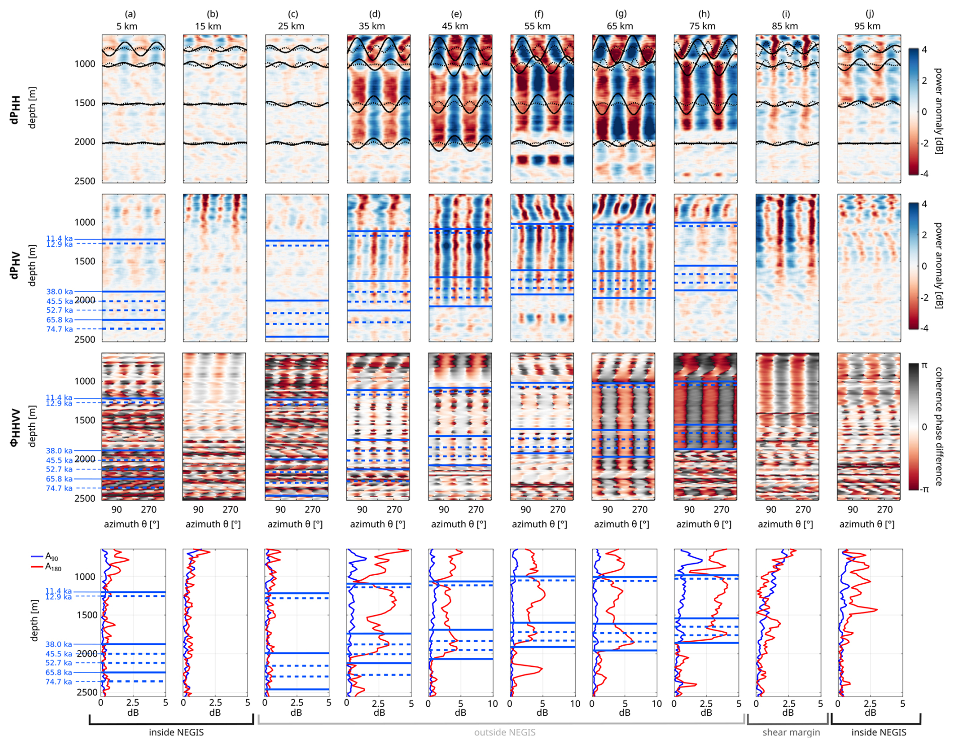
Figure 5 Synthesized azimuthal radar response for profile B: top panels show the co-polarized power anomaly dP_HH with the fitted 90°- and 180°-periodic sine curve shown as dotted and solid lines, respectively, at depths of 800, 1000, 1500, and 2000 m. Middle panels show the cross-polarized power anomaly dP_HV and coherence phase difference ϕ_HHVV. The x axis on each panel in the upper three rows shows the azimuth rotating clockwise from true north. Bottom panels show the amplitudes (in decibel) of the 90 and 180° periodic signal component with depth. Notice the different x axes of the bottom panels. Blue horizontal lines indicate the depths of isochrones traced in Fig. 7.

The periodicity in the CoPE indicates whether anisotropic scattering or birefringence is dominating the radar response. Among all analysed points and depths, 80 % are dominated by anisotropic scattering, and at 57 % of these points, the 180° periodicity is twice as strong as the 90° periodicity. The lowest scattering dominance is found close to the shear margins and at intermediate depths (∼630–1500 m), where 59 % of the analyses within less than 3 km from the shear margins are dominated by a 180° periodicity. However, deriving strength and orientation of anisotropic scattering and birefringence in the vicinity of the shear margins is particularly difficult due to the overall decreased radar return power related to strongly folded layers. Abrupt changes in the scattering amplitudes often, but not always, coincide with the 11.4 ka isochrone depth indicating the Wisconsin–Holocene transition that is , for example, visible in the amplitude–depth profiles in Figs. 4a and f–i and 5d–h.

The orientation of the XPE in the cross-polarized power anomalies can indicate COF rotations (Ershadi et al., 2022). A notable azimuth rotation occurs at a depth of 1200–1400 m between 55 and 75 km in profile A (Fig. 4f and h), where the XPE is rotated by up to 45°. XPE azimuth rotations also appear particularly pronounced in profile B at 35 km and 55–65 km at depths between 1000 and 1300 m, possibly indicating a COF rotation (Fig. 5d, f, and g). Notably, the depths where these XPE rotations occur coincide with the depth of the 11.4 ka isochrone for all these examples, and in profile B they go along with an additional change in scattering orientation at the Wisconsin–Holocene transition.

The coherence phase reveals 90°-periodic dipole nodes, which, unlike CoPE nodes in dP_HH, remain distinguishable as individual features even in the presence of anisotropic scattering. Anisotropic scattering primarily reduces the angular width of these nodes, providing an alternative indication of scatter strength (Ershadi et al., 2022). Anisotropic scattering appears, for instance, particularly strong at 5–55 km, 95 km in profile A (Fig. 4a–f and j), and 35–55 km in profile B (Fig. 5d–f). The vertical spacing between coherence phase nodes further visually indicates the degree of horizontal COF anisotropy in the survey area, corresponding to differences in horizontal eigenvalues. The integrated phase difference can in theory be used to derive horizontal eigenvalue differences, a method which works reliably in low-anisotropy areas (e.g. Jordan et al., 2022; Young et al., 2021). However, for strong COF anisotropy the depth differences between reflections of opposite polarization directions exceed the radar's range resolution, leading to loss of coherence (Zeising et al., 2024). Although the phase coherence method could not be applied successfully to our dataset for deriving COF eigenvalues, reprocessing the data to reduce radar bandwidth might improve its applicability in future efforts, albeit at the cost of signal strength (Zeising et al., 2024).

Figure 6 shows the orientation of the 180° periodic signal at depths of 800, 1000, 1500, and 2000 m, along with the apparent horizontal eigenvalue difference. The eigenvalue difference was determined using an automated process that measures the travel-time difference between the HH and VV traces. Specifically, the cross-correlation of each trace pair was calculated within a 20 m sliding window to estimate the time delay between signals. Linear regression was then applied to correlated reflections to obtain the depth-averaged apparent eigenvalue difference (for method details, see Gerber et al., 2023). The uncertainty of this method increases when only shallow reflections are available or when the number of reflections is low. To ensure reliability, we only included results where at least 10 internal reflections could be correlated with a correlation coefficient above 0.6 and where at least one reflection lies below 1200 m depth. Results were discarded where these criteria were not met, particularly in areas with steeply dipping internal layers near shear margins.

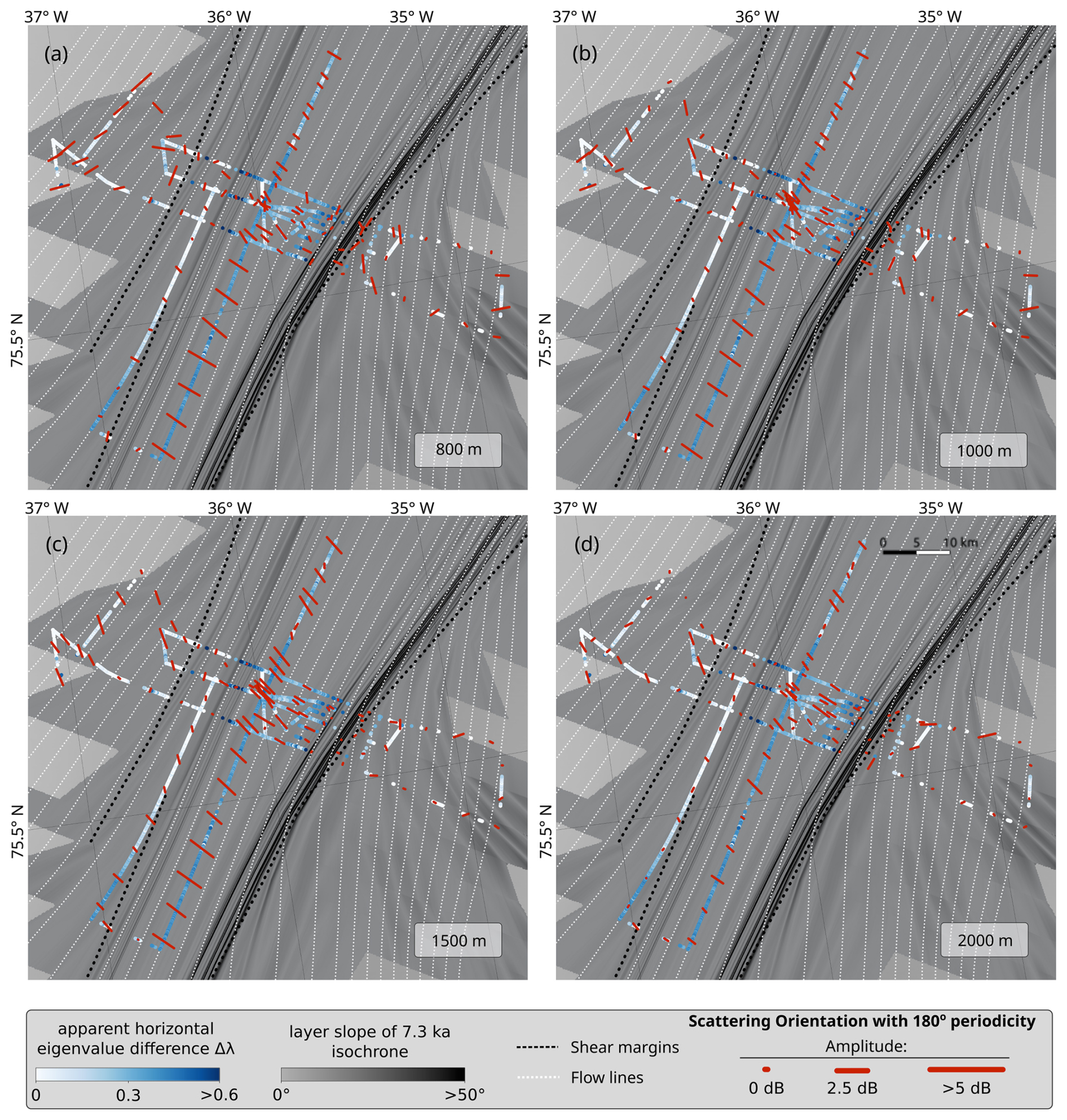
Figure 6 Orientation and amplitude of anisotropic scattering at a depth of (a) 800, (b) 1000, (c) 1500, and (d) 2000 m. The orientation (depicted by line orientation) and strength (depicted by size) of scattering are obtained from the amplitude A₁₈₀ and phase φ₁₈₀ of the 180°-periodic component in Eq. (2), which has been fitted to dP_HH. White-to-blue colours along the radar lines indicate depth-averaged apparent horizontal eigenvalue difference derived from HH–VV travel-time differences. The background depicts the slope of the 7.3 ka isochrone from Jansen et al. (2024), highlighting regions of pronounced folding where travel-time differences failed to reveal reliable eigenvalue differences.

The scattering direction in the ice-stream centre is oriented between 95 and 105° clockwise from the surface flow direction at depths of 1000–1500 m where scattering is strongest. Near the shear margins, scattering becomes less dominant and the orientation rotates, which is particularly visible in profile A, following close to the southwestern shear margin in Fig. 6. This rotation of scattering direction coincides with and explains the apparent reduction in horizontal anisotropy derived from travel-time differences, as HH and VV wave speed differences are maximized when aligned with the COF and minimized when misaligned. Outside the shear margins, the scattering orientation is close to flow-parallel at shallow depths (Fig. 6a) but rotates by approximately 90° for larger depths (Fig. 6b and c), notably in profile B in the northwestern corner of Figs. 6 and 5 at 35–75 km.

This reversal of scattering direction is also visible in the HH–VV power difference of the radargrams, demonstrated for profiles A and B in Fig. 7, which shows that the power difference clearly follows the ice-sheet stratigraphy. Positive (blue) values indicate increasing return power perpendicular to the driving direction, while negative (red) values indicate increased power parallel to the driving direction. For along-flow profile sections inside the ice stream (e.g. A1–A2, B1–B2, B4–B5), power differences tend to be positive in most parts of the ice column, indicating that the power return approximately perpendicular to ice flow (HH) is up to 10 dB stronger. Profile parts that were recorded perpendicular to ice flow (e.g. A2–A3, B2–shear-margin, B7–B1) show a negative power difference, confirming that more energy is scattered in the direction perpendicular to the flow (in this case VV). A notable change occurs at the 11.4 ka isochrone, marking the Wisconsin–Holocene climatic transition. Inside the ice stream (e.g. the 0–40 km section of profile A and the 0–10 km section of profile B), this transition is marked by an increasing HH–VV power difference, while outside the shear margins (20–70 km of profile B) the sign of the power difference is reversed. In this same section of profile B, a folded unit between the 65.8 and 74.7 ka isochrones is also characterized by different scattering properties and a reversed scattering direction compared to the overlying ice layers. Sections A3–A4, B2–B3, and B5–B6 show alternating signatures of positive and negative power difference, particularly pronounced in Holocene ice, which is a result of birefringence-induced beat signatures: birefringence causes a rotation of the polarization ellipsoid in and out of the profile plane, so the power alternates between being higher parallel (VV) and perpendicular (HH) to the profile direction. These birefringence-induced beat signatures are indicative of the misalignment of radar antennas and COF principal axes. The fact that strong beat signatures are mostly visible at shallow depths might be due to the loss of coherence at larger depths. In both profiles there is an approximately 200 m thick basal echo-free zone.

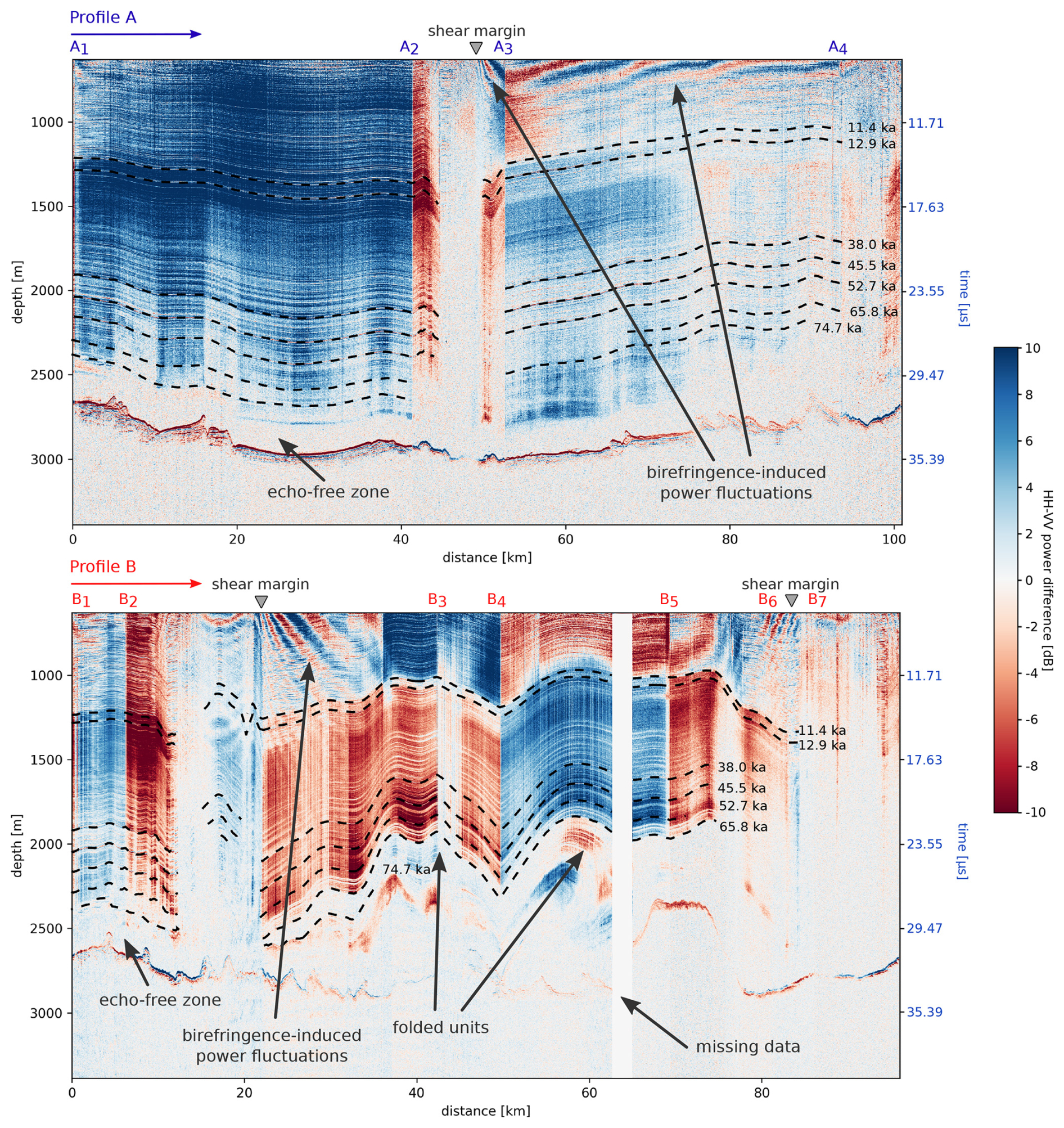
Figure 7 Difference in power return of co-polarized modes (HH–VV). Panels (a) and (b) show profiles A and B in Fig. 1. Turns in the radar lines are marked with A₁–A₄ and B₁–B₇, respectively, and the corresponding locations are indicated in Fig. 1. The driving direction is from left to right. The grey triangles mark the positions of the shear margins outlined in Fig. 1. Dashed lines indicate internal reflection horizons of labelled age. Profile B is missing some data at ∼65 km.

5 Discussion

We observe the presence of both anisotropic scattering and birefringence effects at EastGRIP and in radar lines recorded within a radius of 50 km from the EastGRIP drill site, extending over the entire ice-stream width and beyond the shear margins. Notably, birefringence is most pronounced near the shear margins and at shallow depths but is often superimposed by anisotropic scattering which clearly dominates the azimuthal response in the ice-stream interior and exterior, particularly in ice units dating back to the Wisconsin period. In the following, we first discuss the origin of anisotropic scattering, then examine the relationship between observed backscatter properties and climate-induced ice characteristics, and finally explore the implications of our findings for inferring COF type and orientation.

5.1 Origin of anisotropic scattering

Three potential mechanisms have previously been identified as being most likely causes for anisotropic scattering (Drews et al., 2012): (1) elongated air bubbles, (2) directional interface roughness, and (3) small-scale variations in COF with depth. We next discuss each process separately.

5.1.1 Air bubbles

Air bubbles form near the ice-sheet surface during the transformation of firn into ice. As they are buried under additional snow and ice layers, they compress, causing a reduction in their diameter with depth and deformation under a deviatoric stress regime. The number, size, and shape of bubbles vary between layers deposited under different atmospheric conditions (Svensson et al., 2005), leading to stratification on larger scales. Eventually, bubbles transform into clathrate hydrates (e.g. Miller, 1969; Ohno et al., 2004), a transition that occurs in the range of 500 to 1000 m depth in the EastGRIP ice core (Stoll et al., 2021), and exhibit only minimal variation across the Greenland Ice Sheet (Pauer et al., 1999; Kipfstuhl et al., 2001; Neff, 2014).

Bubbles generally elongate in the direction of dilatational strain (Hudleston, 1977) and can therefore serve as proxies for local strain rates (Alley and Fitzpatrick, 1999). Highly elongated bubbles are usually found in rapidly shearing layers with orientation parallel to the shear zone (Hudleston, 1977; Russell-head and Budd, 1979). Smaller bubbles are generally more spherical than larger ones, so bubble elongation tends to decrease with depth (Alley and Fitzpatrick, 1999). In central NEGIS, the flow regime is characterized by along-flow extension due to acceleration and flow-transverse compression from lateral inflow, while shearing dominates at the shear margins (Stoll et al., 2024; Westhoff et al., 2021; Gerber et al., 2023). Although direct studies of bubble shape in the EastGRIP ice core are still ongoing, bubbles in the ice-stream centre are expected to be slightly elongated in the flow direction, becoming most elongated in and parallel to the shear margins.

Previous studies (Drews et al., 2012) suggest that elongated air bubbles can cause anisotropic scattering, with increased return power in the direction of bubble elongation. In our survey area, this would imply higher return power along the flow direction and parallel to the shear margins. If bubbles were the sole cause of scattering, we would expect decreasing anisotropy with depth until the clathrate transition at ∼1000 m, along with a slight rotation and stronger anisotropic scattering near the margins, and weaker anisotropic scattering outside the ice stream.

We reject the hypothesis that bubbles are the major cause for anisotropic scattering observed in this study based on three key reasons. First, the spatial distribution of scattering directions and amplitudes does not align with expected scattering caused by bubble elongation in the corresponding strain regimes, although this conclusion is limited by the lack of direct observations. Second, if air bubbles were the dominant cause of anisotropic scattering, we would expect a gradual change in anisotropy with depth, which we do not observe. Finally, while anisotropic scattering occurs throughout most of the ice column, its strength and direction follow the internal stratigraphy of the ice sheet. Although bubble size and shape might correlate with stratigraphy due to differences in climatic properties, bubbles cannot be the primary cause of scattering at depth because they mainly exist in the upper 1000 m and turn into clathrates at around the same depth range, regardless of ice age.

5.1.2 Interface roughness

Evidence for azimuthal-dependent roughness is observed in the visual stratigraphy of the EastGRIP ice core (Westhoff et al., 2021), which shows roughness amplitudes in the order of centimetres or less. Although folding amplitudes are limited by the ice-core diameter, larger folds relevant for radar wavelengths have been shown to prevail (Jansen et al., 2024). The visual record at EastGRIP shows higher interface roughness perpendicular to the surface flow field (Westhoff et al., 2021), with folding axes aligned parallel to ice flow due to transverse flow compression and along-flow extension in the ice-stream centre. Folding amplitudes increase toward the shear margin and remain parallel to the margin (Jansen et al., 2024).

The effect of directional interface roughness on radar return power is complex. Interface roughness can transition radar signals from specular reflection to more diffuse scattering and wave depolarization when roughness amplitudes are comparable to the radar wavelength (Peters et al., 2005; Giannopoulos and Diamanti, 2008). Studies with side-looking radars have shown that higher backscatter occurs perpendicular to the folding axis, as folds act as corner reflectors (Bateson and Woodhouse, 2004; Bartalis et al., 2006). However, for a nadir-looking radar system with a much narrower beamwidth, this anisotropic scattering mechanism may not operate in the same way. Instead, stronger co-polarized scattering might occur parallel to the folding axis, depending on fold size and radar characteristics (Scanlan et al., 2022).

Despite the unclear relationship between folds and anisotropic scattering, we can rule out directional interface roughness as the major source of anisotropic scattering for the following reasons. First, if directional interface roughness results from ice dynamics, particularly lateral strain, we would expect layers outside the ice stream to be smoother, with less pronounced anisotropic scattering. Indeed, the scattering amplitude is generally slightly higher inside the ice stream than outside (Fig. 6). However, this pattern is not consistent. For example, scattering amplitudes outside NEGIS in profile B exceed the amplitudes in the ice-stream interior, particularly downstream of EastGRIP and in profiles which are not in the ice-stream centre (Fig. 6a–c). Although roughness outside the current ice stream might be a remnant of previous ice-dynamics configurations, the spacial distribution of scattering amplitudes is difficult to explain by roughness alone, particularly the lower amplitudes toward ice-stream margins where folding amplitudes are known to increase (Jansen et al., 2024). Second, while scattering differences between ice from different climate periods could stem from variations in folding amplitudes associated with viscosity differences, the reversed directionality of anisotropic scattering between Holocene and Wisconsin ice north of the NW shear margin would imply an exceptionally distinct strain history between these ice units if attributed to ice-flow-induced interface roughness, which is unrealistic.

5.1.3 Small-scale vertical variation of COF

After ruling out the above mechanisms as the primary origin of anisotropic scattering, we propose that small-scale fluctuations in COF with depth are the most likely cause of the anisotropic scattering observed in our survey area, consistent with Drews et al. (2012) suggesting a similar explanation for anisotropic scattering in other regions. Figure 8 provides a conceptual sketch illustrating how COF variations could explain these observations.

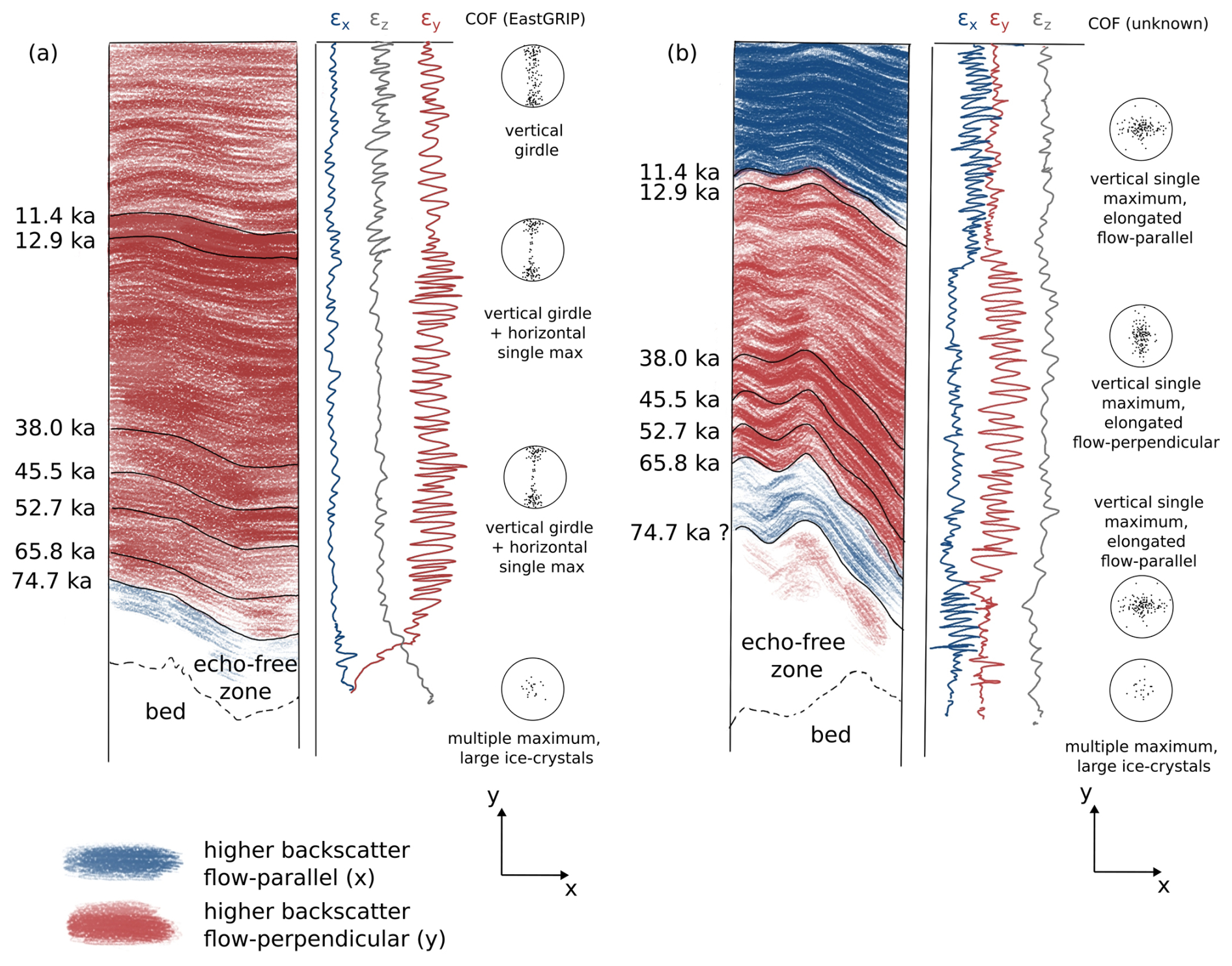
Figure 8 Proposed mechanisms by which COF fluctuations might cause anisotropic scattering: (a) within the NEGIS (where COF is observed in the EastGRIP core) and (b) in folded ice northwest of NEGIS. Red indicates higher backscatter in the flow-perpendicular direction, whereas blue indicates backscatter in the flow-parallel direction. The anisotropic scattering arises not from the COF type itself but from its vertical fluctuations, which influence horizontal relative permittivities (ε_x,y). In (a), a vertical girdle with a superimposed horizontal single maximum dominates most of the ice column. We suggest that fluctuations in the single maximum's strength in the flow-perpendicular direction drive the increased flow-perpendicular scattering. In (b), the COF type is unknown, but travel-time differences suggest types with minimal horizontal anisotropy. Anisotropic scattering may arise from COF fluctuations where the orientation with maximum eigenvalue fluctuation reverses at climatic transitions – for instance, a vertical single maximum with slight elongation toward the flow-parallel or flow-perpendicular directions in different ice units. In both scenarios, a basal echo-free zone is observed, characterized by very large crystals with multi-maxima COF. This likely accounts for the absence of both anisotropic scattering and radar echoes in this layer.

Panel (a) depicts the scenario within the ice stream, where COF characteristics are well-constrained by the EastGRIP core (Stoll et al., 2024). Across most depths relevant to the radar, a vertical girdle dominates, with eigenvalues primarily distributed in a plane perpendicular to the flow direction. The flow-parallel eigenvalues remain near zero and show only minor variations with depth. Consequently, the flow-parallel dielectric permittivity remains relatively constant with depth. In contrast, the flow-perpendicular eigenvalues are generally larger and exhibit greater fluctuations with depth, impacting the flow-perpendicular permittivity toward larger variations. These eigenvalue fluctuations lead to a reflection coefficient of up to 15 dB (Sect. S1) and anisotropic scattering with increased return power perpendicular to ice flow, which is in agreement with the observed HH–VV power difference of roughly 10 dB in the ice-stream interior. We hypothesize that the discrepancy between the COF-derived scattering coefficient and radar-measured values could stem from the relatively large measurement intervals of the COF (5–15 m).

Notably, scattering amplitudes increase slightly at the Wisconsin–Holocene transition within the NEGIS. Stoll et al. (2024) document that at this transition in the EastGRIP core (1230–1394 m) the vertical girdle develops into a girdle with an asymmetrical two-maxima COF. Afterwards, an additional horizontal maximum component arises together with the girdle and prevails down to 2500 m with varying strength. These observations clearly show COF changes at the Wisconsin–Holocene transition, and even though the overall COF type and horizontal eigenvalue differences remain nearly the same, the increased scattering amplitude in Wisconsin ice can be explained by higher permittivity fluctuations due to the varying strength of the single maximum. Additionally, Stoll et al. (2024) observe that below 2500 m ice crystals grow significantly larger due to elevated temperatures and organize into a multi-maxima COF with predominantly vertical orientation. This aligns well with the echo-free zone and explains why anisotropic scattering is only observed above this layer.

Panel (b) in Fig. 8 represents the situation in the folded units north of NEGIS. Here, no direct COF observations are available from ice cores, so the permittivity profile and stereoplots in panel (b) are speculative. Apparent eigenvalue differences derived from travel times are small, suggesting either low horizontal anisotropy or a misalignment of the COF with radar polarization. Assuming that strain outside NEGIS is dominated by vertical compression, a vertical single-maximum COF is the most likely configuration, resulting in low horizontal eigenvalue differences. Nevertheless, anisotropic scattering could still arise from such a COF if the c axis distribution (and thus the dielectric permittivity) varies more in the flow direction within the upper Holocene ice unit. This pattern could then shift to greater flow-perpendicular permittivity variation in the Wisconsin ice. This COF rotation would also explain the azimuth change in XPE, which coincides with the Wisconsin–Holocene transition in Fig. 5.

5.2 Relation between anisotropic signatures and climate- and strain-induced properties of the ice

We find that scattering strongly follows the ice-sheet stratigraphy, as highlighted by the HH–VV power difference in Fig. 7, which reveals ice units with distinct scattering properties. The reversal in scattering orientation between Holocene and Wisconsin ice in the folded ice north of NEGIS is particularly striking, but similar observations have been reported elsewhere. For example, Horgan et al. (2008) identified a distinct seismic reflectivity boundary at Sermeq Kujalleq (Jakobshavn Glacier or Jakobshavn Isbræ in Danish), interpreted as the transition between Holocene and Wisconsin ice. Likewise, Wang et al. (2018) observed layers in Antarctica with different seismic scattering properties that correspond to distinct climatic periods.

A similar reversal in scattering orientation is observed in the folded ice between the 65.8 and 74.7 ka isochrones in profile B (Fig. 7). This unit is characterized by intact and continuous internal reflection horizons and weaker anisotropic scattering with the same directionality as Holocene ice. In contrast, the overlying Wisconsin layers and folding axes exhibit reversed scattering orientation. The age of this folded unit remains uncertain, as ambiguities in tracing deep isochrones, particularly the 74.7 ka isochrone, across the shear margin complicate age estimates. If the reversal in scattering orientation here results from mechanisms similar to those at the Wisconsin–Holocene transition, it is plausible that the folded ice originates from the last warm period, the Eemian. If so, this ice is considerably older (>120 ka) than the oldest isochrone we traced, suggesting disrupted and possibly inverted stratigraphy caused by folding – a phenomenon also observed in other regions of the Greenland Ice Sheet (e.g. Suwa et al., 2006; NEEM Community members, 2013).

In Fig. 8, we proposed a potential mechanism for the reversed scattering pattern, though we do not claim to fully explain the formation of these COF differences. Ice from colder periods, like the Wisconsin, tends to have a higher impurity content and smaller crystals, promoting easier deformation compared to ice from warmer periods like the Holocene and Eemian (Paterson, 1991; Cuffey et al., 2000; Faria et al., 2014b, a). The folding of ice itself does not inherently produce a 90° rotation of COF needed to invert the scattering signature. However, changes in the regional ice dynamics could have altered the local strain regime to which the COF adjusts accordingly. The rate and manner of this adjustment may differ between ice units, with Wisconsin ice, having generally higher impurity content and smaller grains, potentially adjusting more rapidly or distinctly than Holocene ice, which could explain the observed scattering differences.

Our findings have significant implications for glaciological research and palaeoclimate reconstruction. Quad-polarized radar data that distinguish ice units based on scattering properties enhance our understanding of ice-sheet dynamics and structure. For instance, identifying ice units with varying micro-scale properties, such as basal shear zones, could improve ice-sheet models by incorporating depth-dependent variations in mechanical properties – an aspect often assumed constant throughout the ice column. Additionally, scattering properties aligned with ice-sheet stratigraphy could aid automated routines for tracing internal horizons. If scattering properties can be linked to climate-induced microstructure, quad-polarized radars could also help identify ages of ice units and detect inverted stratigraphy, which is critical for palaeoclimate studies and selecting ice-core drilling sites. It remains for future studies to investigate how anisotropic scattering relates to climatic transitions in other regions of ice sheets and to explore the reliability of using these scattering properties to map ice extent and microstructural characteristics across different climatic periods.

5.3 Implications on inferring COF type and orientation

In addition to COF type and strength, its orientation is crucial in order to understand bulk effects on ice dynamics. Cross-polarized power anomalies (dP_HV) can indicate COF orientation, in particular in combination with the phase coherence gradient (Jordan et al., 2019) but can be challenging when the COF rotates with depth (Ershadi et al., 2022). In our analysis, the rotation of XPE in some parts (Figs. 4 and 5) suggests some sort of COF rotation. However, the interpretation is not straightforward due to integrated path effects (Zeising et al., 2023), as a rotation of, say, 45° does not necessarily imply a 45° rotation of the COF axes.

The direction of anisotropic scattering can give an independent indication of the COF orientation when scattering origins other than COF can be ruled out. The 180° periodic signal in the ice-stream centre is rotated clockwise from the flow direction by 95–105°, suggesting that the eigenvectors are not perfectly aligned with the surface flow as has been commonly assumed (Westhoff et al., 2021; Gerber et al., 2023), a conclusion which was also reached by Nymand et al. (2025) using double reflections to derive COF orientation from the same dataset as this study. A notable rotation of the scattering direction is also shown in the second-half of profile A (55–100 km in Figs. 4 and 6), located in the vicinity of the shear margin, where the scattering axes are rotated 20–70° clockwise, with a tendency toward stronger rotation at larger depths. Here again, Nymand et al. (2025) found similar results. The COF rotation here explains the apparent decrease in horizontal anisotropy derived from travel-time differences, which does not represent the true anisotropy in case of misalignment of COF axis and radar wave polarization. The agreement between scattering COF orientation derived by Nymand et al. (2025) further supports our conclusion that scattering can be attributed to COF orientation, which has the advantage of being independent of depth and strength of anisotropy and observable at any orientation of the quad-polarized measurement.

It is worth noting that care should be taken in areas of strongly folded internal stratigraphy, particularly in our study area in the vicinity of the shear margins. Here, the overall return power is decreased because of steep internal layers. Hence the smaller scattering amplitudes do not necessarily imply smaller COF fluctuations with depth but may simply reflect the overall decreased return power. Although birefringence effects are mostly found to be dominant near the shear margins and at relatively shallow depths, anisotropic scattering still dominates in most of the analysed cases.

While scattering orientation can act as an independent measure for the orientation of COF principal axes when other scattering sources can be ruled out, it can also complicate efforts to derive COF strength from RES measurements. Previous studies used airborne RES surveys with a standard co-polarized antenna configuration to derive the horizontal eigenvalue difference from the vertical spacing of CoPE nodes (Young et al., 2021; Gerber et al., 2023). The presence of strong anisotropic scattering expands CoPE nodes in the vertical (e.g. Ershadi et al., 2022), which makes the identification of individual nodes challenging while also affecting the azimuth angle at which CoPE appears strongest. Anisotropic scattering could be one reason why this method proved to be difficult inside the NEGIS (Gerber et al., 2023), with another reason being the loss of coherence for larger depths due to strong anisotropy. Similar challenges appear in analyses of CoPE in polarimetric RES measurements. Horizontal eigenvectors and differences in horizontal eigenvalues can also be derived from the coherence phase, which is more robust to anisotropic scattering but is limited in its ability to detect abrupt COF changes (Jordan et al., 2019) and strong fabric anisotropy with high bandwidths (Zeising et al., 2023). Ultimately, inverse methods as suggested by Ershadi et al. (2022) are a valuable tool to approximate the full orientation tensor of the COF. However, well-defined initial conditions are crucial, and the inversion is challenging when COF rotation with depth is significant. Decomposing the co-polarized power anomalies into its 180- and 90°-periodic components can help with constraining the initial conditions in both scattering magnitude and the presence of COF rotation with depth for such inversion efforts in the future.

6 Conclusions

We used curve-fitting methods to analyse the relative importance of anisotropic scattering and birefringence on the azimuthal power response in ground-based quad-polarized RES data collected in the NEGIS onset region. We found that the 180° periodic effect of anisotropic scattering dominates the co-polarized power anomaly in 80 % of the analysed locations and depths, while the 90° periodic signal of birefringence tends to be only dominant at depths of less than 1000 m and near the shear margins. We conclude that small-scale COF fluctuations, i.e. its variance or noise, with depth is the most likely cause of anisotropic scattering and that the scattering direction is likely aligned with one horizontal eigenvector. Scattering properties strongly follow the ice-sheet stratigraphy, indicating the potential to use quad-polarized measurements to identify ice units with different scattering properties, e.g. basal zones or ice from cold/warm climatic periods.

Our results are in agreement with previous studies which found anisotropic scattering being dominant over birefringence in highly dynamic areas, while the opposite is observed in slow-moving locations of ice sheets. This leads to challenges in deciphering the COF strength and direction from co- and cross-polarized extinction, and we leave a full inversion of quad-polarimetric data as proposed by Ershadi et al. (2022) for future work. While we are confident that anisotropic scattering is mostly related to COF here, it remains unclear how other physical parameters like impurity content and crystal size affect these scattering mechanisms in different ice units and different areas of ice sheets. Continuous high-resolution COF measurements of ice cores as well as larger-scale airborne polarimetric RES surveys would be beneficial for understanding the scattering properties of climatic transitions and mapping their distribution in ice sheets.