A facet-based numerical model to retrieve ice sheet topography from Sentinel-3 altimetry

In this study, we present a facet-based numerical model dedicated to ice sheet radar altimetry. The model simulates Sentinel-3 UnFocused-Synthetic Aperture Radar (UF-SAR) waveforms by calculating the backscattered radar signal over the 10 m facets of the Reference Elevation Model of Antarctica (REMA). The simulation is exploited to determine the coordinates of the impact point on the ground, where the surface elevation is estimated. The complete processing chain, named the “Altimeter data Modelling and Processing for Land Ice” (AMPLI), provides topography estimations posted at ∼330 m along the satellite track. Using ICESat-2 as a reference mission, we evaluated the performance of the AMPLI software over the Antarctic ice sheet. The median bias between Sentinel-3 AMPLI and ICESat-2 ATL06 nearly co-located measurements is estimated at +12 cm on average over the Antarctic ice sheet. This surface height difference exhibits spatial variations over the Antarctic ice sheet, of the order of few decimetres. These divergences are most likely induced by the terrain characteristics (slope and roughness) and snow volume scattering affecting Ku-band altimetry measurements. The performance improvement is substantial compared to the ESA level-2 products, in particular over the ice sheet margins. For example, where the surface slope is greater than 0.5°, the median bias and the median absolute deviation relative to ICESat-2 ATL06 are reduced by about 83 % and 90 %, respectively. We also assessed the capability of Sentinel-3 to monitor surface elevation change (SEC) over the Antarctic ice sheet. The comparison between SEC maps from Sentinel-3 AMPLI and ICESat-2 ATL15, calculated over the 2019–2022 period, shows a Pearson correlation of 0.92. The study highlights the benefit of radar signal modelling, in synergy with high-resolution digital elevation models (DEMs), for reducing the slope-induced errors over ice sheets. The results emphasise the potential of the Sentinel-3 constellation for ice sheet mass balance studies.

1 Introduction

The Antarctica and Greenland ice sheets are critical areas to monitor, given their current and projected contributions to sea level rise (IPCC, 2023: Ocean, Cryosphere and Sea Level Change). Over the past decades, satellite radar altimetry has proved to be one of the most widely used techniques to achieve this goal (Otosaka et al., 2023; Shepherd et al., 2020). Among the contemporary altimetry missions monitoring the cryosphere, Sentinel-3 is an Earth observation satellite series developed in the frame of the European Copernicus programme. Sentinel-3 is jointly operated by the European Space Agency (ESA) and EUMETSAT, to deliver operational ocean and land observation services (Donlon et al., 2012). The mission objectives include the delivery of geophysical products containing, among others, land ice surface elevation. At the time of writing, the Sentinel-3 constellation includes two satellites: Sentinel-3A and Sentinel-3B, launched on 16 February 2016 and 15 April 2018, respectively. Both spacecraft are positioned on a high-inclination orbit, covering polar areas up to a latitude of about 81.5°. Consequently, Sentinel-3 samples the Greenland ice sheet almost entirely and a large part of the Antarctic ice sheet. The two Sentinel-3 units perform equivalently over ice sheets, as reported in McMillan et al. (2021).

Among its payload, Sentinel-3 carries the dual-frequency Synthetic aperture Radar ALtimeter (SRAL). The altimeter sends radar pulses at high frequency (∼18 kHz) to exploit the Doppler effect induced by the satellite movement (Raney, 1998). As implemented in the ESA Copernicus Ground Segment (CGS), the UnFocused Synthetic Aperture Radar (UF-SAR) processing generates measurements with a footprint of about 330 m in the along-track direction. Several studies demonstrated the advantages of delay-Doppler altimetry for ice sheet monitoring, in comparison to conventional low resolution mode (LRM) (Aublanc et al., 2018; McMillan et al., 2019). Most notably, as a result of the smaller footprint size, the slope-induced error affecting ice sheet radar altimetry is reduced. In fact, over ice sheets the surface topography derived from radar altimeters is not estimated at nadir but commonly “relocated” at the expected impact point on ground. This point is generally located in the upslope direction: termed in the literature as the “point of closest approach” (POCA) (Brenner et al., 1983).

In comparison with the CryoSat-2 mission, Sentinel-3 does not have interferometric capabilities to autonomously geolocate the radar returns on the ground. Therefore, a priori knowledge of the surface topography must be used for that purpose, namely a digital elevation model (DEM). Several methods have been developed over time to perform the echo relocation over ice sheets. One of the first developed techniques determines the POCA in the orthogonal direction to the surface, assuming a constant slope in the radar footprint (Brenner et al., 1983; Cooper, 1989). Another alternative approach finds the POCA by searching for the shortest range between the satellite and the DEM nodes (Roemer et al., 2007). This method was refined by restricting the relocation procedure within the actual area sampled by the waveform leading edge (Li et al., 2022; Huang et al., 2024).

In this study, we present the “Altimeter data Modelling and Processing for Land Ice” (AMPLI). The software is a level-2 processing chain dedicated to Sentinel-3 altimetry measurements acquired over ice sheets. It includes a new relocation method, performed by means of an innovative numerical modelling of the radar waveform. The AMPLI software is described in the first section of this paper. In the second section, the Antarctic ice sheet elevation estimated with the AMPLI processing is evaluated against the ICESat-2 ATL06 product. In the third section, the 2019–2022 surface elevation change (SEC) of the Antarctic ice sheet, derived from Sentinel-3 AMPLI topography estimates, is evaluated against the ICESat-2 ATL15 product. In the last section, we investigate the observed differences between Sentinel-3 and ICESat-2 over the Antarctic ice sheet interior and discuss perspectives for improvement.

2 Altimeter data Modelling and Processing for Land Ice (AMPLI)

2.1 Motivation and overview

Since the 2000s, a new generation of ice DEMs appeared, based on the photogrammetric processing of optical images acquired from different viewing angles (Toutin, 2002; Berthier et al., 2014). Through this technique, the Polar Geospatial Center (PGC) released the Reference Elevation Model of Antarctica (REMA) in 2018, the first continental-scale DEM available at a resolution of less than 10 m (Howat et al., 2019). The motivation for developing the AMPLI software was to take advantage of the high resolution of REMA, with the aim of using it in a facet-based model dedicated to ice sheet radar altimetry. Among the possible applications for this model, we identified the development of a new relocation method as a top priority. In fact, for conventional altimeters operating in LRM, the slope-induced error is recognised to be by far the main contributor to the error budget over the polar ice sheet margins (Brenner et al., 2007). This statement remains true for Sentinel-3 delay-Doppler altimetry (McMillan et al., 2019).

The end objective of the AMPLI software is to derive the surface topography from Sentinel-3 UF-SAR altimetry measurements acquired over ice sheets. The topography is estimated at 20 Hz along the satellite orbit and is relocated in the cross-track direction, in general at the POCA. The 20 Hz posting rate implies that two consecutive elevation estimates are separated by an along-track distance of about 330 m on the ground. The AMPLI software comprises two main modules:

• “Facet-based simulation” module. Based on orbital and instrumental data read in the ESA Land Ice Thematic Products, Sentinel-3 UF-SAR waveforms are simulated along the satellite track with a facet-based numerical model, described in Sect. 2.2.

• “Retracking and Relocation” module. The ice sheet elevation is estimated with a retracking algorithm adapted from the Leading Edge Detection (LED) algorithm (Aublanc et al., 2021). The horizontal coordinates of the measurement are estimated at the point of first radar return, as described thereafter in Sect. 2.3. This relocation is performed using the outputs from the facet-based simulation.

In terms of input altimetry data, the processing starts with the level-2 Sentinel-3 Land Ice Thematic Products, Baseline Collection no. 5. The products are operationally generated and distributed by ESA since September 2023 from the Copernicus Data Space Ecosystem (CDSE) facility. A full mission reprocessing was accomplished prior to the operational deployment, providing a homogeneous and complete data set to the users (Sentinel-3 Mission Performance Cluster consortium, 2024). In terms of input auxiliary data, the altimetry measurements are selected over the Antarctic ice sheet and ice shelves, by means of the surface mask from the BedMachine data set, version no. 3, for Antarctica (Morlighem et al., 2020). The facet-based simulation is performed using the REMA DEM, 10 m resolution, version no. 2, released in 2022 (Howat et al., 2019).

2.2 Numerical facet-based simulation

In 1977, Brown proposed an analytical formulation of the radar echo over a rough sea surface, based on the convolution from the flat surface impulse response (FSIR), the probability density function (PDF) of the scatterer heights and the system point target response (PTR) (Brown, 1977). In this work, we start from the same FSIR formulation and discretised it at the DEM grid points. Hence, through this so-called “facet-based simulation”, the effect of terrain roughness is integrated into the radar signal modelling down to decametre-scale variations. After simulation of the energy backscattered over the radar footprint, the delay-Doppler processing performed on ground is reproduced to generate synthetic UF-SAR waveforms. A summary of the calculations is provided below, with additional details available in Sect. S1 in the Supplement. The validity of the Brown model over the ice sheet surface is also discussed in Sect. S1. It is worth noting that a similar facet-based approach was developed in the recent past for sea ice (Landy et al., 2019) and ice sheet (Helm et al., 2024) radar altimetry.

As mentioned, the processing takes a level-2 Sentinel-3 Land Ice Thematic Product as input. Several variables of this product are required for the simulation, among them the satellite altitude, the nadir coordinates and the altimeter tracker range. Other parameters used in the Retracking and Relocation module are also extracted, in particular the UF-SAR waveform and a set of geophysical corrections needed for the surface elevation computation. For each 20 Hz record selected within the BedMachine mask, a subset of the DEM is extracted, centred at nadir. In this study, we performed the modelling over a relatively large area of 35 km×35 km. This allows almost all the energy from the antenna main lobe to be simulated, as the −10 dB antenna beamwidth projected on the ground extends up to ∼16 km from nadir. The geometric calculations are performed in Cartesian coordinates (x,y), using the Antarctic Polar Stereographic projection (EPSG:3031). The equations take into account the Earth's curvature.

The energy backscattered at the snow–air interface P_fs(x,y) is computed for each facet of the DEM, following the FSIR formulation (Brown, 1977):

$$\begin{array}{}\text{(1)}& P_{\text{fs}}(x,y)={\displaystyle \frac{\mathit{\lambda }{\mathit{\sigma }}_{\mathrm{0}}}{(\mathrm{4}\mathit{\pi }{)}^{\mathrm{3}}}}\underset{A}{\int }\left({\displaystyle \frac{G^{\mathrm{2}}\left(\mathit{\theta }\right)}{r^{\mathrm{4}}}}\right)\mathrm{d}A,\end{array}$$

where λ is the radar wavelength, σ₀ is the backscattering coefficient of the surface, A is the area of a surface facet, r is the distance between antenna and the facet, and G(θ) is the antenna pattern modelled with a Gaussian function (the mathematical formulations of these variables are reported in Sect. S1). As Brown (1977), we ignored the variation of backscattering coefficient with angle of incidence. This simplification was made to facilitate and speed up the numerical calculations and is further discussed in Sect. S1.

The modelling was designed to generate amplitude radar signals, without considering the phase information. The processing does not simulate radar pulses at pulse rate frequency (PRF) but directly emulates 2D delay-Doppler maps (DDMs) at 20 Hz rate. This speeds up the computational time and avoids speckle noise in the waveforms. The DDMs are constructed by integrating the backscattered energy P_fs(x,y), given the facet–satellite distance in slant range (range–time domain, t) and in the along-track direction (Doppler frequency domain, f).

In the range–time domain (t), a range gate index R_i is attributed to the DEM facets, given the satellite–facet distance and the onboard tracker command. This index corresponds to the relative position of the DEM facet in the window analysis, which comprises 128 range gates for SRAL:

$$\begin{array}{}\text{(2)}& R_i(x,y)=\left({\displaystyle \frac{r-T_{\mathrm{r}}}{\mathit{\alpha }}}\right)+R_{\text{ref}},\end{array}$$

where α is the altimeter vertical resolution, T_r the altimeter tracker range, and R_ref the reference index of the tracker range in the window analysis.

In the Doppler frequency domain (f), 64 iso-Doppler coordinates are determined across the satellite track for each of the 64 beams constituting the DDM. Each delay-Doppler frequency is separated by an along-track distance corresponding to the azimuth resolution achieved in UF-SAR (∼330 m on average). In addition, a histogram of the energy backscattered is constructed for each delay-Doppler beam as a function of (a) the cross-track distance between the facet and the ground track and (b) the slant-range distance between the facet and the satellite. We call this signal the cross-track backscatter distribution (CTBD), which is further used in the relocation processing presented in Sect. 2.3.

Figure 1 provides an example of DDM and CTBD generated for a Sentinel-3 measurement located in Marie Byrd Land, West Antarctica. In this example the surface slope is estimated at 0.6°, mainly in the cross-track direction. Therefore, the iso-range lines from the R_i matrix (in white) are shifted upslope and do not have a perfect circular disc shape due to the topography variations over the radar footprint. The Doppler beams are constructed by interpolating the backscattered energy P_fs(x,y) along the corresponding iso-Doppler lines across the satellite track (in cyan). This interpolated energy is classified as a function of the cross-track distance in the CTBD, for each delay-Doppler frequency. In Fig. 1, the CTBD corresponding to null Doppler frequency (f_i=0) is represented.

Figure 1 (a) Topography from REMA over which the simulation is performed (only a 20 km×20 km area is represented). The white contours display the iso-range lines R_i, the cyan lines represent the 64 delay-Doppler frequencies. (b) Energy backscattered at the snow–air interface P_fs. (c) Delay-Doppler map simulated by integrating the energy P_fs along the iso-Doppler frequencies, given the satellite–facet distance in slant range. (d) Cross-track backscatter distribution, showing the histogram of the energy P_fs in the cross-track direction, along the Doppler frequency index no. 0.

Once the DDMs are generated along the satellite track, a second loop is performed on the 20 Hz records to produce the delay-Doppler stacks. To this end, the delay-Doppler beams (taken from different DDMs) sampling the same surface on the ground at different viewing angles are gathered together. In the ESA ground segment processing, the delay-Doppler stacks comprise 180 delay-Doppler beams, or single looks, from DDMs available at 80 Hz. In this processing, as the DDMs are emulated at 20 Hz, an equivalent number of 45 single looks are kept in the delay-Doppler stacks. The multi-looking operation is performed with an extended window, following the ground segment specification (Sentinel-3 Instrument Processing Facility team, 2023). This processing has been implemented since Baseline Collection no. 5 to optimise the data coverage over steeply sloping topography (Aublanc et al., 2018). Finally, a numerical convolution is applied between the UF-SAR waveform and the range PTR.

2.3 Retracking and relocation procedures

Figure 2 displays the conceptual flow chart of the retracking and relocation procedures implemented in the AMPLI software. These algorithms are in general included in the ground segment level-2 processing.

Figure 2 Flow chart describing the main operations included in the “Retracking and Relocation” module implemented in the AMPLI software.

The retracking algorithm outputs the round-trip delay between the antenna and the surface into the “altimeter range” parameter. The estimated altimeter range is compensated for additional delays due to the ionosphere and troposphere and for effects due to the solid Earth tide, pole tide and ocean loading tide. These geophysical corrections were extracted from the Sentinel-3 Land Ice Thematic Products. The retracking operation is performed using the Leading Edge Detection (LED) algorithm, initially developed for SARIn CryoSat-2 measurements. This algorithm was inspired from the Canny edge detector (Canny, 1986) to identify waveform energy peaks in a radar altimetry waveform and is described in Aublanc et al. (2021). The retracking point, or epoch position, is estimated in the first waveform leading edge identified by the LED algorithm, at peak half-power. This approach is analogous to the Threshold First Maximum Retracking Algorithm (TFMRA), developed by Helm et al. (2014).

For most of the Antarctica measurements, the backscattered energy contributing to the first energy peak originates from the POCA. Nevertheless, we found that this assumption is not always true due to the presence of complex irregular topography, or the behaviour of the onboard tracker or both (see example in Fig. 5c). Therefore, in this paper, we use a more general terminology of “point of first radar return” to refer to the coordinates where the measurement is relocated.

Figure 3 illustrates the main operations performed during the relocation processing, using a measurement selected over the ice sheet margins as an example. As displayed in Fig. 3a, the relocation algorithm takes two signals generated during the numerical modelling, presented in Sect. 2.2, as input: the simulated UF-SAR waveforms and the CTBD. A cross-correlation is first performed between the Sentinel-3 UF-SAR waveform and the simulated waveform:

$$\begin{array}{}\text{(3)}& \begin{array}{rl}& {\text{WF}}_{\text{xcorr}}\left[k\right]=\sum _{i=\mathrm{0}}^{N-\mathrm{1}}{\text{WF}}_i\times {\text{SWF}}_{i-k+N-\mathrm{1}}^{\ast }\\ & \text{for }k=\mathrm{0},\mathrm{1},\mathrm{\dots }N-\mathrm{1},\end{array}\end{array}$$

where i is the waveform index, N is the number of range gates, WF is the Sentinel-3 UF-SAR waveform and SWF is the simulated waveform. Both WF and SWF signals are normalised by their respective maximum value, as displayed in Fig. 3.

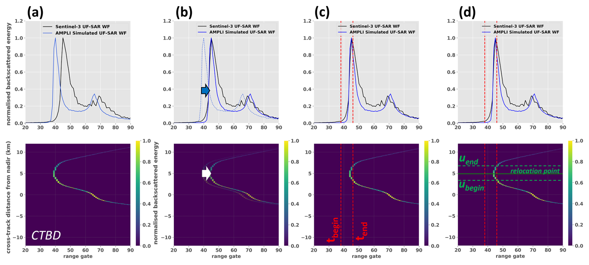
Figure 3 Illustrations of the relocation procedure implemented in AMPLI, with, on the top, the simulated (blue) and measured (black) Sentinel-3 UF-SAR waveforms, and on the bottom the cross-track backscatter distribution (CTBD), which represents the histogram of the energy backscattered in the cross-track direction. (a) The input signals. (b) The CTBD is readjusted in slant range, given the cross-correlation delay between the simulated and measured UF-SAR waveforms. (c) The dotted red lines show the start and stop gates of the waveform leading edge, as identified by the retracker. (d) The measurement is relocated at the centre of gravity (solid green line) of the cluster area, as highlighted between dotted green lines.

The simulated waveform and CTBD are aligned to the Sentinel-3 UF-SAR waveform in the range–time domain, by applying the cross-correlation delay (Fig. 3b). This operation was set up to correct for a vertical offset in the DEM, as discussed in Sect. 5.2. The cross-track footprint sampled by the waveform first energy peak is estimated in this delayed CTBD. To this end, the part of the signal included between t_begin and t_end is extracted in the range–time domain. The range gates t_begin and t_end correspond to the start and stop gates of the waveform leading edge, as identified during the retracking procedure (dotted red lines in Fig. 3c).

A clustering segmentation is performed in the extracted CTBD to determine the distinct across-track areas illuminated by the waveform energy peak. The facet clusters are simply detected by joining together the adjacent CTBD across-track index with non-null energy. When the surface is relatively flat and smooth, as observed in the ice sheet interiors, the first waveform leading edge is generally shaped with backscattered energy originating from one single cluster. But over more irregular topography, multiple distinct clusters can contribute to the energy peak. In the latter situation, the measurement is relocated at the most powerful cluster, provided that its integrated power contributes to at least 50 % of the waveform energy peak. In the case of more than two detected clusters, if no cluster is found to be predominant, the measurement is flagged as “ambiguous”. In addition, an ambiguity is considered if the cross-track extension of the identified cluster (i.e. the distance between u_begin and u_end) extends beyond 6 km. In both situations of surface ambiguity, the measurement is flagged. These ambiguous measurements were discarded in the evaluations presented in Sects. 3 and 4.

The cross-track surface finally considered sampled by the waveform leading edge is delimited by the u_begin and u_end indexes (dotted green lines in Fig. 3d). A centre of gravity (COG) computation is performed on the selected cluster to determine the cross-track position of the point of first radar return in this selected cluster (solid green line in Fig. 3d):

$$\begin{array}{}\text{(4)}& {\text{COG}}_{\text{CTBD}}={\displaystyle \frac{{\sum }_{u_{\text{begin}}}^{u_{\text{end}}}\left(n\times \left({\sum }_{t_{\text{begin}}}^{t_{\text{end}}}\text{CTBD}[t,u]\right)\right)}{{\sum }_{u_{\text{begin}}}^{u_{\text{end}}}\left({\sum }_{t_{\text{begin}}}^{t_{\text{end}}}\text{CTBD}[t,u]\right)}}.\end{array}$$

COG_CTBD provides the cross-track distance (in metres) between nadir and point of first radar return. This information is employed to geolocate the point of first radar return on a polar stereographic plane (EPSG:3031). The look angle between nadir direction and point of first radar return is computed as

$$\begin{array}{}\text{(5)}& \text{look angle}=\text{arccos}\left({\displaystyle \frac{\mathrm{\Delta }\mathit{H}\cdot \mathrm{\Delta }\mathit{R}}{\mathrm{\Delta }H\times \mathrm{\Delta }R}}\right),\end{array}$$

where ΔH is the distance between satellite and nadir, and ΔR is the distance between satellite and the estimated point of first radar return.

$$\begin{array}{}\text{(6)}& \begin{array}{rl}& \mathrm{\Delta }H=\sqrt{(x_{\mathrm{s}}-x_{\mathrm{n}}{)}^{\mathrm{2}}+(y_{\mathrm{s}}-y_{\mathrm{n}}{)}^{\mathrm{2}}+(z_{\mathrm{s}}-z_{\mathrm{n}}{)}^{\mathrm{2}}};\\ & \mathrm{\Delta }R=\sqrt{(x_{\mathrm{s}}-x_{\mathrm{r}}{)}^{\mathrm{2}}+(y_{\mathrm{s}}-y_{\mathrm{r}}{)}^{\mathrm{2}}+(z_{\mathrm{s}}-z_{\mathrm{r}}{)}^{\mathrm{2}}},\end{array}\end{array}$$

where ($x_{\mathrm{s}},y_{\mathrm{s}},z_{\mathrm{s}}$), ($x_{\mathrm{n}},y_{\mathrm{n}},z_{\mathrm{n}}$) and ($x_{\mathrm{r}},y_{\mathrm{r}},z_{\mathrm{r}}$), are the coordinates of satellite, nadir and point of first radar return, respectively, in the Earth-centred, Earth-fixed (ECEF) frame.

With the knowledge of both the look angle and the altimeter range parameters, the surface topography can be estimated in the cross-track plan. This is achieved with geometric calculations performed in ECEF, the same ones as employed in Aublanc et al. (2021). At the end of the processing, the agreement between the simulated and the Sentinel-3 UF-SAR waveforms is controlled, as described in Sect. S3.

2.4 Illustrations

Figure 4 shows Sentinel-3A UF-SAR waveforms generated by the ESA ground segment processing, along a track portion located in the West Antarctic Ice Sheet. The measurements were acquired in July 2022. The track segment displayed is about 250 km length. This example was selected to illustrate a scenario where the ground segment produced complex UF-SAR waveforms, containing multiple energy peaks. The waveforms simulated with the AMPLI software are represented below the ground segment processing ones. The visual comparison indicates that the AMPLI software correctly reproduced the radar UF-SAR waveforms over this track segment. A more quantitative assessment is provided in Sect. S2, demonstrating the overall validity of the facet-based simulation in the Antarctic ice sheet.

Figure 4 Illustration of the Sentinel-3A waveforms generated by the ESA ground segment processing (a) and simulated with the AMPLI software (b), along a track portion of about 250 km length, located in West Antarctica. The segment displayed is highlighted in red in panel (c). The dotted red lines correspond to three single measurements used as case studies to illustrate the relocation processing in Fig. 5.

In Fig. 5, we provide three case studies, along the track segment displayed in Fig. 4, to illustrate the relocation processing implemented in AMPLI. In the first case (Fig. 5a), two distinct clusters are found contributing to the energy peak identified during the retracking operation. In this situation, the measurement is relocated at the most powerful cluster, as previously described. In the second case, a multi-peak waveform is shown (Fig. 5b). The first significant leading edge is generated with energy coming from POCA, where the measurement is relocated. In the third case (Fig. 5c), a low-energy peak arises from the POCA, located ∼4.5 km from nadir, which cannot be detected by the retracker. However, thanks to the developed methodology, the point of first radar return is consistently positioned within the area sampled by the first significant energy peak.

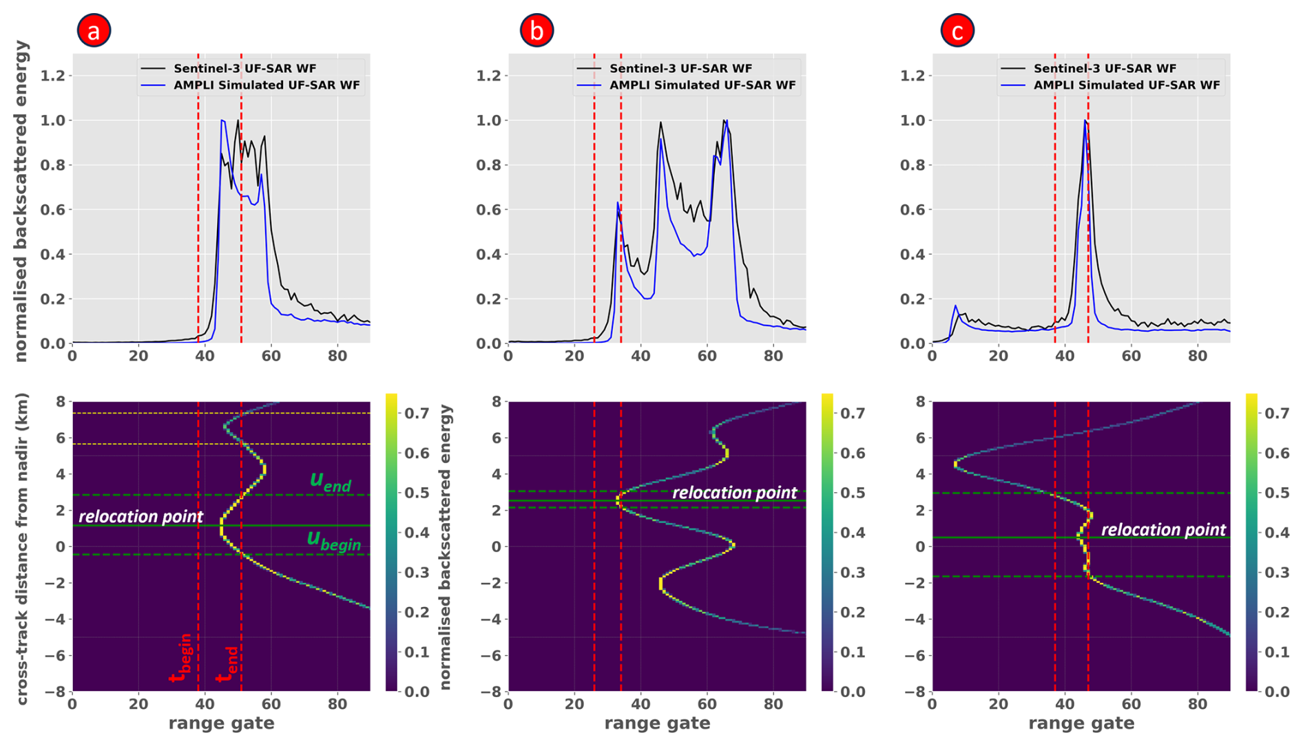
Figure 5 Illustration of the relocation method implemented in the AMPLI software, for three case studies (a–c). Sentinel-3A UF-SAR waveforms (black) and AMPLI-simulated waveforms (blue) are displayed in the top panels. The corresponding AMPLI cross-track backscatter distributions (CTBDs) are displayed in the bottom panels. Dotted green lines delineate the identified clusters for the relocation (i.e. the cross-track areas considered sampled by the waveform leading edge). Solid green lines indicate the centres of gravity of the cluster areas where the measurements are relocated. In the case of (a), dotted yellow lines delineate the location of an ambiguous cluster.

3 Evaluation of ice sheet elevation

3.1 Sentinel-3 data set

Sentinel-3A and Sentinel-3B measurements acquired in Antarctica from 9 May to 25 August of 2019 were processed with the AMPLI software. The period covers 108 d, corresponding to four full orbit cycles of 27 d duration. The middle of the period coincides with the ICESat-2 ATL15 timestamp to compare the Sentinel-3 and ICESat-2 SEC estimations, presented in Sect. 4, as closely as possible. Approximately 27 million Sentinel-3 measurements were selected over the Antarctic ice sheet, as defined in the BedMachine surface mask. The ice sheet elevation estimated by the ESA ground segment processing, and available in the level-2 Land Ice Thematic Product, was also assessed (product variable “elevation_ocog_20_ku”). We use the terminology “ESA L2” to refer to this data set in the text. In the ESA ground segment, the relocation method assumes a linear slope to determine the POCA. The surface slope is extracted from slope models, themselves derived from auxiliary DEMs produced by Helm et al. (2014). The relocation algorithm was initially developed for LRM altimetry and is described in Scott et al. (2007). It was further adapted to the geometry of delay-Doppler altimetry for the usage in the Sentinel-3 ground segment. The ESA L2 altimeter range is estimated with the OCOG/ICE-1 retracker (80 % threshold) (Wingham et al., 1986).

Common quality controls were applied to both the Sentinel-3 ESA L2 and the AMPLI data set. The elevation retrievals that deviate by more than 50 m to REMA were discarded, as well as measurements relocated further than 15 km from nadir. The acquisitions with low signal-to-noise ratio (SNR) were also rejected, by means of a backscatter coefficient estimated on the UF-SAR waveforms (see Sect. S3 for details in the rejection procedure). Few additional quality controls were also applied to the AMPLI data set only, based on information from numerical modelling. Firstly, the measurements with ambiguity in the relocation processing are discarded, as described in Sect. 2.3 (∼2.34 % of data rejection). Secondly, the agreement between the Sentinel-3 UF-SAR and the corresponding simulated waveform is also checked (∼0.52 % of data rejection in the case of non-accordance). After quality controls, the ice sheet topography was successfully retrieved from 92.26 % and 90.84 % of the Sentinel-3 ice sheet measurements, for the ESA L2 and the AMPLI data set, respectively. Tables S2 and S3 in the Supplement provide the ratio of discarded measurements for each individual quality test, along with a brief description of the control procedures. An illustration of the surface sampling achieved by the twin Sentinel-3 satellites, over Pine Island drainage basin, is available in Sect. S4.

3.2 ICESat-2 ATL06 data set

Similarly to a previous analysis made with CryoSat-2 SARIn data (Aublanc et al., 2021), we used the ICESat-2 mission to evaluate the performance of Sentinel-3 altimetry over the Antarctic ice sheet. In comparison to radar altimetry, the ICESat-2 footprint size is much smaller (∼13 m) to optimise the surface height retrieval over heterogeneous glaciers (Markus et al., 2017). In this study, we used the ATL06 product (release 006), providing land ice elevations posted at approximately 40 m along the six ground track beams. Over the Antarctic ice sheet interior, the ICESat-2 ATL06 elevations have a reported accuracy and precision of about 3 and 7 cm, respectively (Brunt et al., 2021). Bad-quality data were discarded using the binary “atl06_quality_summary” product flag. As with the Sentinel-3 data set, the spatial selection over the Antarctic ice sheet was performed using the BedMachine surface mask. Overall, approximately 2584 million ATL06 elevation measurements were selected over the Antarctic ice sheet, acquired from 24 March to 10 October of 2019.

3.3 Methods

A point-to-point methodology was employed to compare the Sentinel-3 and ICESat-2 ATL06 elevations, as performed in previous studies (Aublanc et al., 2021; Wang et al., 2015). The elevations from both sensors are compared if the measurements are considered co-located in space and time. A search radius of 25 m was used to find spatial co-located measurements. The maximal time span between the acquisitions was set to ±46 d. With this threshold, the temporal collocation is performed by exploring one full ICESat-2 orbit cycle of 91 d duration. Where multiple ICESat-2 records existed within the space–time research, the closest measurement in space was selected. In total, approximately 1787 and 1750 million co-located measurements were identified over the Antarctic ice sheet, with the ESA L2 and the AMPLI data set, respectively. For each co-located point, the elevation difference is computed as Sentinel-3 minus ICESat-2. No further filtering is applied to the data.

3.4 Results

The bias and dispersion between Sentinel-3 and ICESat-2 elevations were quantified with commonly used statistics: mean, median bias, median absolute deviation (MAD) and standard deviation (SD). These metrics were determined for several slope ranges, as reported in Table 1. The surface slope was computed at a 15 km scale around nadir. The mean and SD statistics were calculated with outliers removed, using the 10th and 90th percentiles. It must be noted that the measurements acquired at latitudes further south than 80° S were not selected in the statistics reported in Table 1. The 80° S value was chosen to keep a relative spatial homogeneity in the measurements analysed, representative of the Antarctic ice sheet. In fact, the population of co-located measurements significantly increases in the southernmost areas due to narrower track spacing. In Fig. 6, the median bias and MAD relative to ICESat-2 ATL06 are mapped using a 40 km stereographic grid with a standard parallel of 71° S (EPSG:3031). The grid resolution was chosen to maximise the spatial coverage, with at least 30 co-located elevations per box.

Table 1 Statistics of the elevation difference between Sentinel-3 and ICESat-2 ATL06 nearly co-located measurements (calculated as Sentinel-3 − ICESat-2) over the Antarctic ice sheet, for different slope intervals. Outliers were removed in the mean and SD statistics, using the 10th and 90th percentiles. The measurements acquired further south than 80° S are not considered in this analysis to mitigate statistical over-representation of southern observations, where the population of co-located measurements significantly increases.

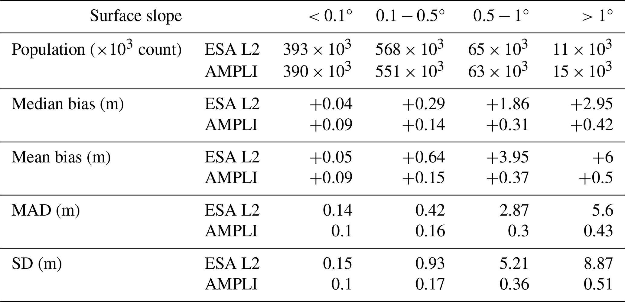
In terms of elevation accuracy, Sentinel-3 and ICESat-2 ATL06 surface heights were found relatively close over low slope areas. Where the surface slope is lower than 0.1°, the median biases relative to ICESat-2 ATL06 are +4 and +9 cm, as obtained with the ESA L2 and the AMPLI data set, respectively. This bias significantly rises over the ice sheet margins in the case of the ESA L2 products. While with AMPLI it remains relatively homogeneous over the Antarctica continent, as it can be seen in the maps in Fig. 6. For example, where the surface slope is greater than 1°, the median bias relative to ICESat-2 ATL06 increases to +295 and +42 cm, for the ESA L2 and the AMPLI data set, respectively. When averaged on a 40 km×40 km map over the Antarctic ice sheet, the median bias between Sentinel-3 AMPLI and ICESat-2 ATL06 remains between ±50 cm for 97.7 % of the grid points. Over the interior of the ice sheet, the median bias between Sentinel-3 and ICESat-2 follows geographical patterns, for both the ESA L2 and the AMPLI data set. These patterns are most likely induced by the spatial variations of snow properties, which are investigated in Sect. 5.1.

Figure 6 Gridded statistics of the elevation differences between Sentinel-3 and ICESat-2 ATL06 co-located elevations: median difference (a, b) and median absolute deviation (c, d). Sentinel-3 elevations were read in the ESA L2 products (a, c) and derived from AMPLI (b, d). Elevations are computed as Sentinel-3 − ICESat-2. Grid resolution is 40 km.

The Sentinel-3 measurement precision is also significantly improved over the ice sheet margins with the AMPLI software, in comparison to ESA L2 products. For instance, when considering all measurements acquired over a slope greater than 0.5°, AMPLI provides an 89.8 % reduction in the MAD relative to ICESat-2. Since the algorithm implemented in the ground segment processing considers a linear slope for the POCA relocation, we assume the methodology is inaccurate in the case of rough surfaces (decametre-/kilometre-scale roughness).

4 Evaluation of surface elevation change

4.1 Sentinel-3 and ICESat-2 ATL15 data set

As mentioned in the Introduction, surface mass balance monitoring is a major application for ice sheet radar altimetry. In general, ice sheet elevation rates are derived from radar altimetry measurements using repeat-track observations of consecutive cycles (Moholdt et al., 2010). Such approaches require continuous time series to be applied. At the time of writing, the AMPLI was too computationally time-demanding for processing the full Sentinel-3A and Sentinel-3B time series within the study timeline. Consequently, it was not possible to use this technique to derive SEC over the whole Antarctic ice sheet. Therefore, we used an alternative methodology to estimate the temporal variation of surface topography, based on elevation residuals calculated against REMA DEM, as described in Sect. 4.2.

Using this approach, SEC was estimated with Sentinel-3 measurements acquired over two separate periods in 2019 and 2022. The 2019 Sentinel-3 data set is the same one as presented and evaluated in Sect. 3.1, with measurements acquired from 9 May to 25 August of 2019. The same time of the year was chosen for the 2022 data set. The initial objective was to avoid, or at least mitigate, seasonal variations of snow properties affecting Ku-band altimeter estimates. Nonetheless, it was shown that temporal variations of snow properties still impact the Sentinel-3 SEC retrieved in the frame of this study. This issue is investigated and discussed in Sect. 5.1. As with the 2019 data set, approximately 27 million measurements from both Sentinel-3A and B units were selected over the Antarctic ice sheet. After quality control, 92.34 % and 90.89 % of the measurements were kept for the analyses of the ESA L2 and the AMPLI data set, respectively.

The Sentinel-3 SEC estimation was compared to the one available in the ICESat-2 ATL15 product, release 003 (Smith et al., 2023). The ATL15 product provides time-varying estimates of land ice topography, gridded in polar-stereographic projection. The SEC maps are calculated every 3 months, at different spatial resolutions. In our analysis, we extracted the period from 2 July 2019 to 2 July 2022 and used the 10 km grid resolution product.

4.2 Sentinel-3 surface elevation change calculation

The Sentinel-3 SEC was calculated with the following methodology:

• For each Sentinel-3 20 Hz elevation record, a “surface height anomaly” (SHA) value was computed, corresponding to the elevation difference between Sentinel-3 and REMA (10 m version). The DEM value is bi-linearly interpolated at the altimetry coordinates.

• The 20 Hz along-track SHA estimations were averaged on the ICESat-2 ATL15 stereographic grid by taking the median value. No editing or filtering was applied during this gridding operation. Per grid box, 30 samples minimum were required for the computation. This simple data gridding can likely be improved in the future.

• Two SHA grids were produced using SHA retrievals dated from the 2019 and 2022 periods, respectively. The difference between the 2022 and 2019 SHA grids provides an estimation of the SEC over the 3-year period. The SEC is computed over all the Antarctic ice sheet drainage basins, as defined by Zwally et al. (2012).

This method is similar to McMillan et al. (2019), as it makes use of a static auxiliary DEM as a reference surface, against which elevation anomalies are computed to retrieve the height temporal variations. Additionally, Sentinel-3 SEC was also estimated with a second method to confirm the results achieved. In this alternative approach, SEC is derived using Sentinel-3 and ICESat-2 ATL06 measurements co-located in space and separated by 3 years in time. The two SEC estimations were found to be in a high agreement, as presented in Sect. S5. The advantage of the method described in this section is that it provides denser SEC grids, as all valid Sentinel-3 along-track measurements contribute to the SEC calculation, while with the second method only a relatively small proportion of the measurements can be co-located in space with ICESat-2 ATL06 elevations.

4.3 Results

With the methodology set up, the areas covered by the SEC grids are about 8 428 000 and 8 571 000 km², with the ESA L2 and the AMPLI data set, respectively. This represents 70.9 % and 72.1 % of the Antarctic ice sheet surface, respectively. The numbers increase to 89.8 % and 91.4 % if only areas above 81.5° south are considered, approximately the southern latitude reached by the Sentinel-3 orbit. Missing grid points in the Sentinel-3 SEC maps can be observed in two main scenarios: firstly, over East Antarctica as a consequence of wider track spacing with the increased latitude, and, secondly, over the ice sheet margins due to onboard tracking failures or noisy radar waveforms that are considered unusable (i.e. in the case of low SNR or no energy peak detected). As documented in the 2023 annual performance report written by the Sentinel-3 Mission Performance Cluster (MPC), about 9 % of the Antarctic ice sheet measurements are reported as either being missing or having low quality, with most of them located in the in the ice sheet margins (Sentinel-3 Mission Performance Cluster consortium, 2024).

The 2019–2022 SEC maps derived with Sentinel-3 ESA L2 and AMPLI elevations are displayed in Fig. 7, as well as the ICESat-2 SEC grid extracted from the ATL15 product. The main same patterns can be observed in the ICESat-2 ATL15 and Sentinel-3 AMPLI maps. For instance, the two maps depict the ice losses over Pine Island, Thwaites and Getz drainage basins in West Antarctica, while positive elevation variations are seen in Droning Maud Land or Princess Elizabeth Land in East Antarctica. In the Sentinel-3 SEC map derived with ESA L2 surface height estimates, the main SEC patterns remain noticeable, but the information is significantly noisier, in particular over the ice sheet margins. Over the interior of the East Antarctic Ice Sheet (EAIS), the Sentinel-3 SEC exhibits geographical patterns that are not visible in the ICESat-2 ATL15 map. These differences are likely induced by the snow volume scattering effect. This problematic is discussed in Sect. 5.1.

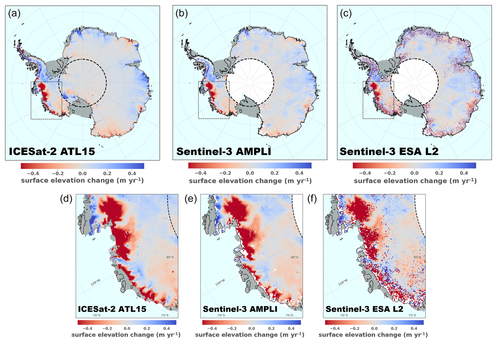
Figure 7 Surface elevation change (SEC) of the Antarctic ice sheet over the 2019–2022 period. SEC is read from the ICESat-2 ATL15 product (a) and is estimated with Sentinel-3A and Sentinel-3B measurements processed by AMPLI (b) and processed by the ESA ground segment (c). (d–f) Same panels but with a zoomed-in view of West Antarctica. Grid resolution is 10 km.

We performed several statistical analyses to evaluate the agreement between SEC maps from Sentinel-3 and ICESat-2 (Fig. 8). Firstly, the relationship between the grid points is displayed in scatter plots (Fig. 8a). The Pearson correlation coefficients (PCCs) obtained are 0.3 and 0.92, as estimated with SEC from the ESA L2 and the AMPLI data set, respectively. The difference between Sentinel-3 and ICESat-2 SEC maps is displayed as a histogram in Fig. 8b (calculated as Sentinel-3 minus ICESat-2). The SDs of the distributions are 49.8 and 6.5 cm yr⁻¹, as obtained with Sentinel-3 ESA L2 and AMPLI SEC maps, respectively. Sentinel-3 AMPLI and ICESat-2 ATL15 SEC maps are within 2 and 10 cm yr⁻¹ agreement for 40.4 % and 93.4 % of the grid points, respectively. These values decrease down to 25.9 % and 73.3 % when Sentinel-3 ESA L2 SEC is compared to ICESat-2 ATL15. The mean bias and MAD between the grid points were also calculated as a function of the surface slope (Fig. 8c). The results confirm the visual interpretation, showing that the SEC derived with Sentinel-3 AMPLI data remains relatively comparable to ICESat-2 ATL15, regardless of the surface slope. In contrast, when Sentinel-3 SEC is estimated with ESA L2 data, the dispersion relative to ICESat-2 ATL15 strongly increases with the slope.

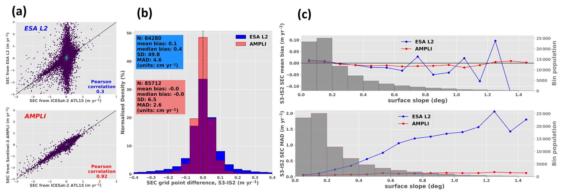
Figure 8 Statistical analysis of the difference between Sentinel-3 and ICESat-2 surface elevation change (SEC) maps of the Antarctic ice sheet, for the 2019–2022 period. In the case of Sentinel-3, SEC is estimated with ESA L2 (blue) and AMPLI (red) data. In the case of ICESat-2, SEC is extracted from the ATL15 product. SEC is mapped on the same 10 km×10 km stereographic grid. (a) Scatter plots of the grid point differences. (b) Histograms of the grid point differences, computed as Sentinel-3 − ICESat-2. (c) Mean bias (top) and median absolute deviation (bottom) of the grid point differences, represented as a function of the surface slope.

Overall, the results emphasise the importance of reducing the slope-induced error for estimating a reliable SEC, at least with the methodology used for deriving the SEC from Sentinel-3 elevation measurements. The correction of snow volume scattering should further improve the conformity between Sentinel-3 and ICESat-2 ATL15 SEC, as discussed in Sect. 5.1. Moreover, better agreement with ICESat-2 can likely be achieved by enhancing the gridding method used to derive Sentinel-3 SEC.

5 Discussions

5.1 Investigations over the East Antarctic Ice Sheet interior

This section focuses on the observed differences between Sentinel-3 and ICESat-2 over the EAIS interior, in both surface height topography (reported Sect. 3.4) and SEC (reported Sect. 4.3). As exhibited in Fig. 6, the bias between Sentinel-3 AMPLI and ICESat-2 ATL06 surface height estimations is not homogeneous in the EAIS interior. It shows spatial patterns, reaching about ±30–40 cm in amplitude. The same analysis was also performed with measurements acquired in 2022, at the same time of the year. The elevation bias also depicts spatial variations, in comparable magnitudes, but the geographical patterns are differently distributed in space. These results are available in Sect. S6.

We identified snow volume scattering as the main effect to explain these topography differences and their variations in space and time. As reported in the literature, over the ice sheet surface the Ku-band radar wave penetrates the snowpack. This generates a volume scattering signal adding up to the one backscattered from the surface at the snow–air interface (Ridley and Partington, 1988). In conventional LRM altimetry, the snow volume scattering signal distorts the waveform shape and consequently impacts the derived geophysical parameters (Legresy et al., 2005). In Ku-band UF-SAR, the waveform leading edge is less sensitive to snow volume scattering, compared to LRM altimetry (Aublanc et al., 2018). Nonetheless, to our knowledge, the impact of snow volume scattering is not yet precisely quantified for Sentinel-3 UF-SAR measurements. We also assumed that snow volume scattering more significantly affects Ku-band radar altimetry compared to ICESat-2 laser pulses.

In the frame of this work, a first analysis was done to demonstrate the influence of the snow volume scattering on the topography retrieved from Sentinel-3 UF-SAR estimations. As noticed in previous studies, the Ku-band backscatter coefficient, namely Sigma-0, is one of the altimetry-derived parameters affected by snow volume scattering (Legresy et al., 2005; Remy and Parouty, 2009). We therefore examined the Sentinel-3 UF-SAR backscatter coefficient variations between 2019 and 2022, using Sigma-0 estimations from the OCOG/ICE-1 retracker (Wingham et al., 1986). The Sigma-0 calculated along the track was averaged in a 10 km×10 km grid (same grid as Fig. 7). Two Sigma-0 grids were produced, corresponding to measurements acquired during Antarctic winter in 2019 and 2022 (same periods as those used for the SEC computation). The analysis is restricted to the EAIS interior, where the terrain elevation is above 2500 m, and the surface slope is below 0.2°. The objective was to perform the assessment over regions where slope-induced errors are assumed to be the lowest in Antarctica. We also selected areas where surface topography is stable, with SEC below 5 cm yr⁻¹, based on ICESat-2 ATL15 estimations.

Figure 9a shows the difference between Sentinel-3 AMPLI and ICESat-2 ATL15 SEC maps. We considered ICESat-2 as the reference in the results' interpretation. This implies that the SEC estimated by Sentinel-3 in the EAIS interior is non-uniformly biased, with maximum errors reaching ±10 to 15 cm yr⁻¹, and distributed in geographical patterns. Figure 9b displays the Sigma-0 variations between Antarctic summer in 2019 and in 2022. On average, a slight positive increase in Sigma-0 is noticed in the analysis area, of about +0.44 dB. But the Sigma-0 temporal variation is not spatially homogeneous, with geographical fluctuations showing patterns of several decibels (between −1.3 and +3.4 dB, according to the 1st and 99th percentiles of the distribution).

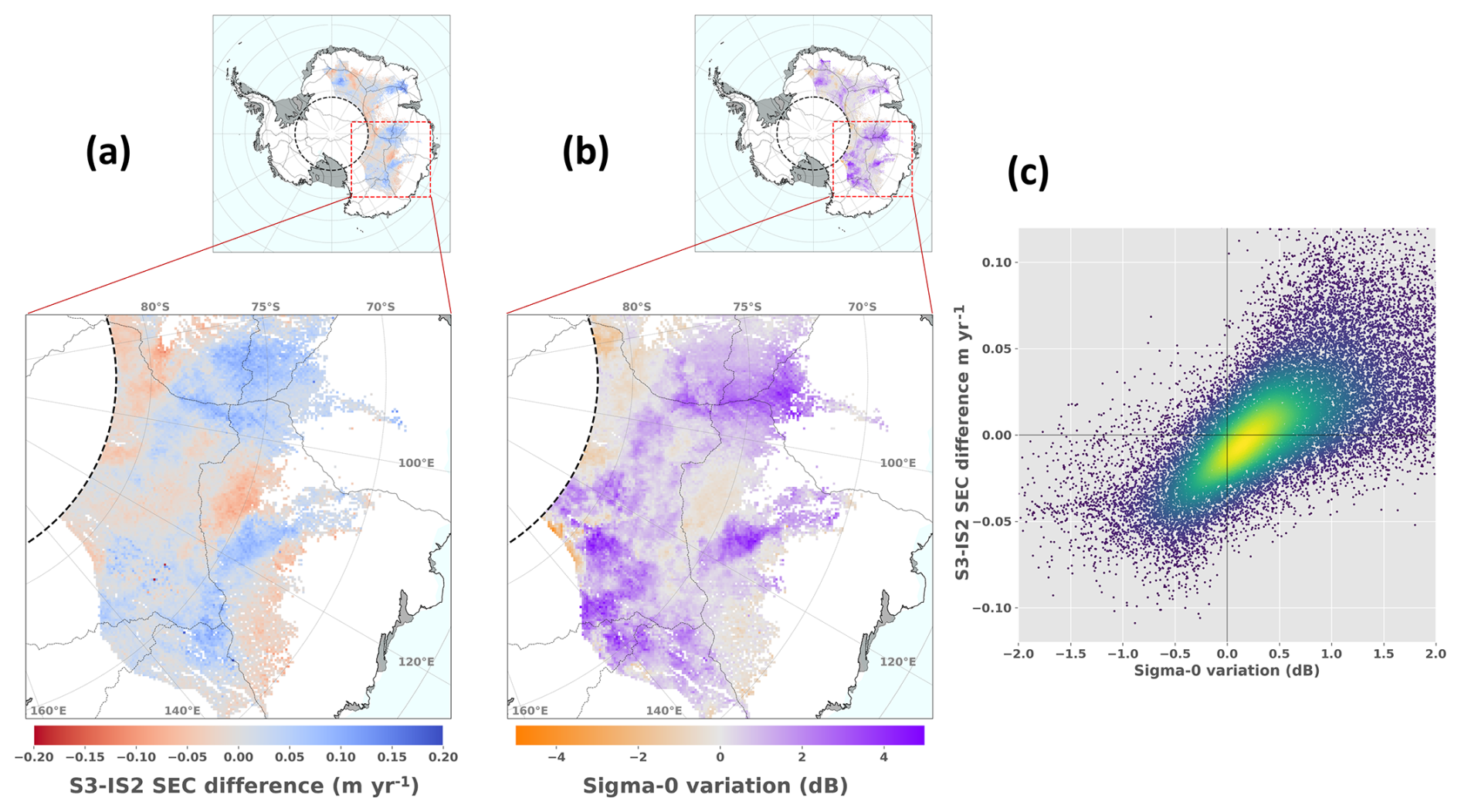
Figure 9 (a) Difference between surface elevation change (SEC) maps from Sentinel-3 AMPLI and ICESat-2 ATL15, calculated over the 2019–2022 period, over the East Antarctic Ice Sheet interior (surface elevation above 2500 m, surface slope below 0.2° and ICESat-2 ATL15 SEC below 5 cm yr⁻¹). (b) Sentinel-3 backscattered coefficient variation between 2019 and 2022 over the same area. (c) Scatter plot between grid points of the Sigma-0 variation map displayed in (b) and SEC difference map displayed in (a).

We analysed the relationship between the Sentinel-3 SEC errors and Sigma-0 temporal variations in the scatter plot displayed in Fig. 9c. A Pearson correlation coefficient of 0.63 is obtained between the two parameters. As observed in the maps Fig. 9, Sentinel-3 SEC appears to be overestimated where the Ku-band Sigma-0 level increases. And conversely, a Ku-band Sigma-0 decrease appears to be associated with a SEC underestimation. The result is consistent with the expectations, as an empirical threshold retracker will estimate a shorter altimeter range in the case of a backscatter coefficient increase (Legrésy and Remy, 1998). This analysis confirms and emphasises the need for a snow volume scattering correction for Sentinel-3 delay-Doppler altimetry. This is further discussed in Sect. 5.3.

5.2 AMPLI assets

We summarise and discuss below the main assets of the AMPLI software, to reduce the slope-induced error affecting ice sheet radar altimetry:

• With the methodology developed, the point of first radar return is detected within the area sampled by the waveform energy peak identified by the retracker, on which the altimeter range is estimated. Thus, the retracking and relocation processing are connected. This concept is also shared by the leading edge point-based (LEPTA) (Li et al., 2022) and MultiPeak Ice (MPI) (Huang et al., 2024) algorithms. As shown in Li et al. (2022), such approaches outperform those making the relocation solely based on the topographical characteristics of the terrain (i.e. without considering the actual surface sampled by the altimeter).

• The relocation method can detect ambiguities in the first radar return, in the case that the energy of the waveform leading edge originates from distinct areas within the measurement footprint. With the facet-based simulation, it is possible to quantify the relative contribution of each area (or cluster) to the waveform energy peak, in terms of backscattered energy.

• The cross-correlation performed between the Sentinel-3 UF-SAR waveform and the numerical model (illustrated Fig. 3b) adjusts for potential vertical bias in the input DEM. To examine the veracity of this statement, positive and negative vertical biases were introduced in REMA (fixed offset), using the same range of values as Huang et al. (2024, Sect. 4.5), up to ±5 m. This analysis is available in Sect. S8. As a result, even with the largest bias values (+5 and −5 m), no performance degradation could be noticed in the surface topography retrieved with the AMPLI software. We consider this is a major advantage in comparison to LEPTA and MPI, as both methods are affected in the case of vertical bias in the input DEM (Huang et al., 2024) and, as a corollary, by temporal surface height variations. This aspect of the processing can be still enhanced, as the echo relocation is however not executed if the vertical bias on the DEM is found higher than ∼14 m (as estimated via the cross-correlation delay between the simulated and the measured waveforms). This evolution is stated among the areas of improvement reported in Sect. 5.3.

• By definition, the echo relocation cannot be accurate anymore in the case of temporal elevation changes that are heterogeneous over the radar footprint. Nevertheless, in such scenarios, it is expected that the waveform simulated with AMPLI will diverge from the altimetry acquisition. Thus, the method developed as the potential to detect and flag such measurements. First procedures were set up to control the agreement between the simulated and the Sentinel-3 UF-SAR waveforms, as presented in Sect. S3.

5.3 Areas of improvement

Among the approximations taken in the numerical modelling described in Sect. 2.2, the main geophysical effect missing is likely the snow volume scattering (Ridley and Partington, 1988). It was outside the scope of this work to explore an accurate modelling for this effect, applicable and validated across the whole of Antarctica. However, previous studies have shown that snow volume scattering has a limited impact on the waveform leading edge in Ku-band SAR mode and rather affects the waveform trailing edge (Aublanc et al., 2018). In Sect. S7, we provide an example illustrating the difference between the measured and simulated Sentinel-3 UF-SAR waveforms over the EAIS interior. Since the volume scattering signal is not yet modelled in AMPLI, the relative energy level of the simulated waveform is lower on the trailing edge part, in comparison to the measured waveform. However, in the relocation procedure developed, the position of the first radar return is estimated within the area sampled by the leading edge part of the waveform only. This likely explains why neglecting snow volume scattering seems to have a limited impact on the Sentinel-3 AMPLI performances, as reported in Sects. 3 and 4. Nevertheless, integrating the snow volume scattering effect into the numerical model remains a priority. It will further improve the agreement between the simulated and measured waveforms. In the current processing, this will be beneficial for better detecting simulation errors. In addition, such modelling enhancement would be used to remove the artificial topography variations induced by temporal changes in the snowpack parameters, as mentioned in Sect. 5.1.

Alongside the numerical modelling aspects, we identify that there are two main different geophysical effects not yet corrected in the developed processing. Firstly, it is critical to compensate for the impact of the snow volume scattering in the altimeter range, which generates errors in the SEC retrieval, as stressed in Sect. 5.1. This can be done by modelling the effect and adding it into the facet-based simulation with the aim of developing a retracking algorithm. Such modelling work has been initiated for LRM altimetry (Lacroix et al., 2008; Larue et al., 2021), but it has never been extensively tested over the entire ice sheet. Alternatively, a post-correction could be added to the elevation retrievals, as commonly done in LRM altimetry using waveform shape parameters (Flament and Rémy, 2012; Simonsen and Sørensen, 2017).

Secondly, we anticipate that the surface roughness, from metre (e.g. sastrugi) to kilometre (e.g. megadunes) scales, would act on the waveform leading edge width. In principle, this would generate errors in the altimeter range because this effect cannot be compensated for by an empirical threshold retracker, as currently implemented in the AMPLI or ESA L2 processing chains. While the associated elevation errors are not yet precisely quantified, we estimate they do not exceed a few decimetres with AMPLI, given the results presented in Sect. 3.4. Furthermore, since such topography features remain relatively temporally static, we also expect these errors to be constant over the time for a given location and therefore to not significantly influence the SEC estimation. Nonetheless, this hypothesis remains to be confirmed. Furthermore, the relationship between the surface roughness (metre to kilometre scales) and the radar waveform shape shall be further assessed, for improving or redefining the retracking algorithm.

Moreover, neural network solutions can also be envisaged to enhance the performance of the AMPLI software. As a first application, these techniques could be employed to better detect modelling errors. In fact, a disagreement between the simulated and measured waveform can for example occur in the case of discrepancies in the input DEM, or heterogeneous elevation change variations over the radar footprint, as discussed Sect. 5.2. A more advanced use would be to develop a neural network retracker, as recently done by Helm et al. (2024). Their retracking solution, named AWI-ICENet1, was applied to CryoSat-2 LRM waveforms acquired over the interiors of the Antarctica and Greenland ice sheets. The results show a reduction in the elevation errors associated with snow volume scattering, compared to other conventional retracking solutions. In parallel to the development of innovative neural network solutions, we also underline the paramount importance to continue improving the radar signal modelling. This is crucial for the efficient and accurate training of neural networks.

Additionally, in the current processing, we decided to tolerate a maximum of ∼14 m elevation difference between the altimetry measurement and the static DEM (as estimated in the cross-correlation, illustrated in Fig. 3b). A future processing evolution could include a dynamic vertical readjustment of the DEM for successfully monitoring regions undergoing rapid elevation changes. Moreover, we set up first quality tests to check the consistency between the simulated and measured waveform. Such procedures can be strengthened to better detect modelling errors or discrepancies in the DEM (occurring in the case of heterogeneous elevation change, as discussed before). To this end, quality control based on machine learning is an option to explore. Finally, a multiple peak retracker would also be valuable to increase the data sampling over the ice sheet margins, as shown in Huang et al. (2024).

6 Conclusion

We developed a numerical model for Sentinel-3 UF-SAR measurements acquired over the Antarctic ice sheet. The modelling is performed through a facet-based simulation by calculating the backscattered radar signal over the 10 m facets of REMA. This model is exploited to relocate the altimetry measurement at its impact point on the ground. The complete processing chain, named the AMPLI software, was assessed in comparison to ICESat-2 standard data products. The median bias between Sentinel-3 AMPLI and ICESat-2 ATL06 nearly co-located measurements is estimated at +12.2 cm on average over the Antarctic ice sheet. This bias exhibits decimetre level variations over the Antarctic continent, most likely induced by the terrain characteristics (slope and surface roughness at different scales), and snow volume scattering affecting Ku-band radar altimetry. When compared to ESA Sentinel-3 Land Ice Thematic Products, AMPLI provides ∼18 % and ∼51 % reductions in the median bias and median absolute deviation relative to ICESat-2 ATL06, respectively. These values increase to ∼83 % and ∼90 %, respectively, where the terrain slope is greater than 0.5°. This demonstrates that the developed processing chain reduces the slope-induced errors affecting ice sheet radar altimetry, in comparison to Sentinel-3 standard product delivered to the users. As expected, the improvements are substantial over the Antarctica coastal areas, where the terrain is steeper and rougher relative to the interior of the continent.

In this study, we also estimated the surface elevation change (SEC) of the Antarctic ice sheet over the 2019–2022 period. The SEC was calculated in a 10 km×10 km map, using surface height retrievals from both Sentinel-3A and Sentinel-3B altimeters, with measurements acquired during the Antarctic winter in 2019 and 2022. The Sentinel-3 AMPLI SEC map covers approximately 72 % of the Antarctic ice sheet and 91 % of the ice sheet area above 81.5° S (southern latitude of Sentinel-3 orbit). The Pearson correlation coefficient between the SEC maps from Sentinel-3 and ICESat-2 ATL15 are 0.3 and 0.92, as obtained with Sentinel-3 elevations from ESA L2 and AMPLI products, respectively. The next priority is to develop a dedicated correction for the snow volume scattering effect. In addition, the processing will have to be assessed over the Greenland ice sheet, ice caps and glaciers. To conclude, this study highlights the potential of the Sentinel-3 surface topography mission for ice sheet mass balance monitoring. With the future launch of Sentinel-3C and Sentinel-3D, the constellation is planned to operate until 2035 at least, which will provide a continuous ∼20-year record of ice sheet observations.