Current reversal leads to regime change in the Amery Ice Shelf cavity in the 21st century

The Amery Ice Shelf (AmIS), the third largest ice shelf in Antarctica, has experienced relatively low rates of basal melt during the past decades. However, it is unclear how AmIS melting will respond to a future warming climate. Here, we use a regional ocean model forced by different climate scenarios to investigate AmIS melting by 2100. The areally averaged melt rate is projected to increase from 0.7 to 8 m yr⁻¹ in the low-emission scenario or 17 m yr⁻¹ in the high-emission scenario in 2100. An abrupt increase in melt rate happens in the 2060s in both scenarios. The redistribution of local salinity (hence density) in front of AmIS forms a new geostrophic balance, leading to the reversal of local currents. This transforms AmIS from a cold cavity to a warm cavity and results in the jump in ice shelf melting. While the projections suggest that AmIS is unlikely to experience instability in the coming century, the high melting draws our attention to the role of oceanic processes in basal mass loss of Antarctic ice shelves in climate change.

1 Introduction

Amery Ice Shelf (AmIS) is a large ice shelf in Antarctica (Fig. 1). It is fed by the Lambert Glacier system, which accounts for about 16 % of the grounded ice in East Antarctica (Allison, 1979). AmIS has a deep grounding line reaching ∼ 2500m below the sea surface (Galton-Fenzi et al., 2008; Yang et al., 2021; Chen et al., 2023), with an in situ freezing point ∼ 2 °C lower than the coldest water mass outside the ice shelf cavity (Galton-Fenzi et al., 2012). This makes AmIS susceptible to ocean temperature changes in the deep ice shelf cavity (Galton-Fenzi et al., 2012; Wang et al., 2022). As ice shelf melt rates respond quadratically to external thermal forcing (Holland et al., 2008), ice with a low freezing point implies that it is more sensitive to any ocean temperature change than with a higher freezing point.

Prydz Bay has a v-shaped coastline and constrains AmIS (O'Brien et al., 2014). It is divided by the Prydz Channel – a trough with a depth of ∼ 500 m at the shelf break – and a deeper trough at the inner embayment named Amery Depression with a bathymetry from 500 to 1000 m (Fig. 1). Fram Bank and Four Ladies Bank are located on the western and eastern sides of Amery Depression and exhibit dramatic differences in zonal topography (Fig. 1). West of Amery Depression, the depth of Fram Bank rises sharply from ∼ 600 to ∼ 200 m over a distance of ∼ 50 km. East of Amery Depression, Four Ladies Bank has a stepwise decrease from a depth of ∼ 200 to ∼ 500 m over a distance of ∼ 200 km (Liu et al., 2018).

High Salinity Shelf Water (HSSW) and modified Circumpolar Deep Water (mCDW) are major water masses causing AmIS basal melting (Galton-Fenzi et al., 2012; Herraiz-Borreguero et al., 2015, 2016). HSSW is a dense and cold (slightly below the surface freezing point) water mass that forms in coastal polynyas within Prydz Bay during sea ice formation (Ohshima et al., 2013; Williams et al., 2016; Portela et al., 2021). When HSSW descends into the AmIS cavity, the temperature of HSSW is higher than the in situ (pressure-dependent) freezing point of seawater in the deepest cavity, which results in a basal melt rate of > 30 m yr⁻¹ at the grounding line (Galton-Fenzi et al., 2012). The resulting meltwater, named Ice Shelf Water (ISW), upwells along the western ice shelf base. ISW, with the temperature of the in situ freezing point, can be supercooled when it is ascending and refreezing beneath the north-western AmIS (Craven et al., 2009).

The cavity under AmIS is presently filled with relatively cold HSSW of −2.2 to −1.8 °C (Craven et al., 2004; Herraiz-Borreguero et al., 2015). This results in relatively low basal melting along with basal refreezing beneath the north-western AmIS (Depoorter et al., 2013; Rignot et al., 2013). Basal melt rates of AmIS have been stable during the past few decades (Adusumilli et al., 2020).

However, Southern Ocean temperatures are projected to increase in a warming climate (Fox-Kemper et al., 2021; Rintoul et al., 2018). Previous studies predict increased upwelling of mCDW onto the continental shelf of the AmIS sector, resulting in a shift in the cavity regime and consequently an increase in basal melting (Naughten et al., 2018; Kusahara et al., 2023; Thomas et al., 2023; Mathiot and Jourdain, 2023). These studies provide insight into the drivers of warming on the continental shelf. For example, a freshening at the surface of Prydz Bay increases vertical stratification and induces warming at depth (Aoki et al., 2022; Thomas et al., 2023; Kusahara et al., 2023). Another mechanism is related to the poleward shift of westerly winds, which enhances the upwelling of mCDW across the shelf break (Spence et al., 2017; Guo et al., 2019; Verfaillie et al., 2022). However, future changes in the links between the warming in Prydz Bay (PB) and the warming in the AmIS ice shelf cavity, i.e. local oceanic currents or intrusive pathways of warm water, still lack investigation.

mCDW was thought to be absent in the AmIS cavity (Craven et al., 2004). However, it has been observed at the AmIS calving front entering the cavity during winter recently (Herraiz-Borreguero et al., 2015). Other hydrographical observations and modelling studies have documented the presence of mCDW on the continental shelf in Prydz Bay (Galton-Fenzi et al., 2012; Herraiz-Borreguero et al., 2015, 2016; Williams et al., 2016; Liu et al., 2017; Guo et al., 2022). The two main pathways of mCDW intruding beneath AmIS are the following:

1. A large cyclonic gyre encircles Amery Depression, known as Prydz Bay Gyre (PBG) (Smith et al., 1984; Nunes Vaz and Lennon, 1996; Heywood et al., 1999). mCDW upwells across the continental shelf, arriving at Prydz Bay over Four Ladies Bank, and is transported by the eastern branch of PBG toward AmIS (Galton-Fenzi et al., 2012; Herraiz-Borreguero et al., 2015; Williams et al., 2016; Liu et al., 2017). Some ISW exits the cavity, recirculates within PBG and returns beneath AmIS (Williams et al., 2016).

2. A narrow current flows between Four Ladies Bank and the eastern coast, named the Prydz Bay Eastern Coastal Current, which originates in the Antarctic Slope Current (Liu et al., 2017, 2018). Due to the step-like deepened bathymetry over Four Ladies Bank, the Antarctic Slope Current is redirected shoreward to conserve potential vorticity, resulting in the formation of the Prydz Bay Eastern Coastal Current (Liu et al., 2018) and bringing mCDW to Prydz Bay (Liu et al., 2017).

Previous studies have documented that a redirected coastal current in front of the Filchner–Ronne Ice Shelf (Hellmer et al., 2017; Naughten et al., 2021) and Ross Ice Shelf (Siahaan et al., 2022) drives a rapid warming of the ice shelf cavity in climate scenarios. The aim of this study is to determine whether the strength and direction of intrusive mCDW pathways in Prydz Bay remain the same or change in response to future climate change and how these changes affect the melt experienced by AmIS.

This paper is structured as follows: Sect. 2 describes our regional model configuration, model forcing and experiments. Section 3.1 presents projections of AmIS basal melting and temperature on the continental shelf. Section 3.2 proposes a mechanism driving the increase in AmIS basal melting. Section 4 presents conclusions and discusses the limits and implications of this work.

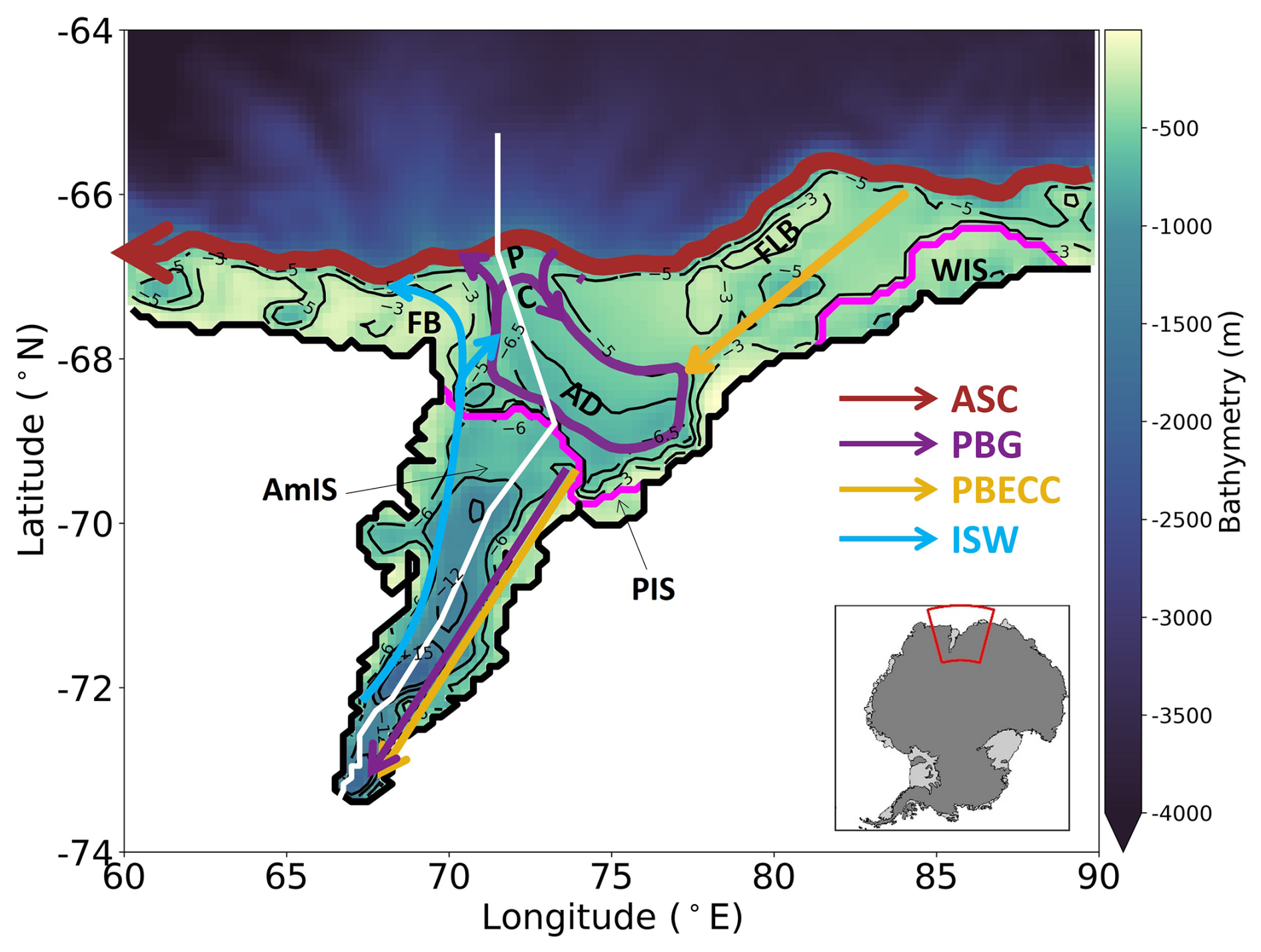
Figure 1 Model domain and schematic diagram of ocean circulation in Prydz Bay. The colour scale shows the bathymetry (m). The thin black lines on the continental shelf indicate the bathymetry of −300, −500 and −650 m. The thin black lines on Amery Ice Shelf (AmIS) show the bathymetry of −600, −800, −1200, −1500 and −2000 m. The thick black line represents the coastal line, and the thick magenta lines show the ice shelf fronts. The thick red arrow represents the Antarctic Slope Current (ASC). The purple arrows show the Prydz Bay Gyre (PBG). The yellow arrow indicates the Prydz Bay Eastern Coastal Current (PBECC). The thin purple and yellow arrows in AmIS show the modified Circumpolar Deep Water. The cyan arrows represent the Ice Shelf Water (ISW). The white line shows a transect extending from the grounding line to the shelf break. The geographical features are labelled as follows: AmIS – Amery Ice Shelf, PIS – Publications Ice Shelf, WIS – West Ice Shelf, PC – Prydz Bay Channel, AD – Amery Depression, FLB – Four Ladies Bank and FB – Fram Bank. Inset: location of AmIS.

2 Models and methods

2.1 Regional model configuration

The regional configuration used to study the Amery Ice Shelf and Prydz Bay (hereafter AME025) is summarized below.

The ocean model used in this study is version 3.6 of the Nucleus for European Modelling of the Ocean (NEMO3.6, Madec et al., 2017). The configuration includes the physical ocean engine OPA (Madec et al., 2017), the sea ice model LIM3 (Rousset et al., 2015) and an open ice shelf cavity (Mathiot et al., 2017). The model domain extends 30° in longitude (60–90° E) and 10° in latitude (65–75° S), with a nominal 0.25° horizontal resolution with grid spacing increasing from ∼ 7 to ∼ 12 km with increasing distance from the South Pole. A 75-level z^* vertical coordinate with a partial cell scheme is used in this work. It is a non-linear free surface application allowing for variations of volume according to the vertical resolution and can adjust at the top and bottom cells to represent bathymetry more realistically. The thicknesses of the grid cells range from 1 m at the surface to 200 m at about 6000 m. Following Global Ocean version 7 (GO7) provided by Storkey et al. (2018), the bathymetry is derived from the ETOPO1 dataset (Amante and Eakins, 2009), with GEBCO giving modifications in coastal regions (IOC et al., 2003). Bathymetry under the ice shelf is derived from IBSCO (Arndt et al., 2013), and the ice shelf draft is taken from BEDMAP2 (Fretwell et al., 2013).

The schemes and parameter values used in the parameterizations are primarily based on a stand-alone global ocean configuration, GO7 (Storkey et al., 2018), but the values of lateral diffusivity and viscosity have been changed according to the smallest grid spacing (∼ 7 km) and time step (720 s). Some physical schemes, such as the slip condition for the lateral boundary, from other regional modelling studies (Mathiot et al., 2017; Jourdain et al., 2017; Bull et al., 2021) are taken into account as well. A 55-term polynomial approximation of the Thermodynamic Equation of Seawater (TEOS-10, IOC et al., 2010) is used in our configuration (Roquet et al., 2015). A vector-form formulation of the momentum advection is applied. The vorticity term is computed using conserving potential entropy and horizontal kinetic energy (Arakawa and Lamb, 1981). Lateral diffusion of tracers is evaluated using Laplacian isoneutral mixing with a coefficient of 135 m² s⁻¹. Lateral diffusion of momentum uses bi-Laplacian geopotential viscosity with a coefficient of −1.08 × 10¹⁰ m⁴ s⁻¹. The vertical eddy viscosity and diffusivity coefficients are calculated from a turbulent kinetic energy (TKE) scheme, with a background vertical eddy viscosity and vertical eddy diffusivity of 1.2 × 10⁻⁴ m² s⁻¹ and 2 × 10⁻⁶ m² s⁻¹, respectively. The enhanced vertical diffusion parameterization is implemented for tracer convective processes with a coefficient of 10 m² s⁻¹. The non-linear bottom friction parameterization is chosen, with a non-dimensional bottom drag coefficient of 2.5 × 10⁻³. The no-slip condition is implemented at the lateral momentum boundary.

Ice shelf thermodynamics are parameterized by the three-equation formulation with velocity-dependent heat and salt exchange coefficients (Jenkins et al., 2010). The top boundary layer thickness is set to 30 m below the ice shelf draft (or the first wet cell if the grid thickness is thicker than 30 m), and the top drag coefficient is set to 2.5 × 10⁻³. The heat and salt exchange coefficients are 1.4 × 10⁻² and 4 × 10⁻⁴, respectively. This implementation does not include external tidal forcing. The velocity of the tidal current at the top boundary is prescribed as 5 cm s⁻¹. A series of sensitivity experiments have been conducted to determine the value of the prescribed tidal velocity (Fig. S1).

2.2 UK Earth System Model (UKESM1.0-LL) forcing

We use climate projections made by UKESM1.0-LL as part of the CMIP6 exercise (Sellar et al., 2020). UKESM1.0-LL is based on the HadGEM3-GC3.1 physical climate model, with additional atmospheric chemistry, and marine and terrestrial biogeochemistry components (Sellar et al., 2020). The ocean model for UKESM1.0-LL is NEMO3.6, and it is based on the 1° Global Ocean version 6 (GO6) configuration (Storkey et al., 2018), with 1° horizontal resolution and 75 vertical levels. The difference between GO6 and GO7 mentioned before is that GO7 is identical to a higher-resolution GO6 0.25° configuration, except that there are open ice shelf cavities in GO7 (Storkey et al., 2018). The differences between the 1 and 0.25° GO6 configurations are the mixing and boundary conditions, which are adjusted according to time step and grid spacing (Storkey et al., 2018).

Model outputs from the first ensemble member (r1i1p1f2) of UKESM1.0-LL have been assessed by previous studies (Beadling et al., 2020; Heuzé, 2021; Purich and England, 2021; Roach et al., 2020; Bracegirdle et al., 2020; Meehl et al., 2020; Forster et al., 2020; Caillet et al., 2024). UKESM1.0-LL is ranked well in terms of various Southern Ocean and Antarctic sea properties (Caillet et al., 2024, Fig. 1). To briefly summarize the evaluations of the modelled Southern Ocean in historical simulations, UKESM1.0-LL has relatively small biases in upper (0–100 m) ocean temperature (Beadling et al., 2020, Figs. 6 and S3), salinity (Beadling et al., 2020, Figs. 6 and S4), bottom temperature (Heuzé, 2021, Fig. A3) and salinity (Heuzé, 2021, Fig. A2) compared to other CMIP6 models. For the interior ocean, UKESM1.0-LL captures temperature and density structure across the continental shelf (Purich and England, 2021, Fig. S2). It exhibits small cold ($<-\mathrm{1}$ °C) and fresh ($<-\mathrm{0.15}$ psu) biases close to the shelf break along the 90° E longitudinal transect (Beadling et al., 2020, Fig. S5), which is the easterly ocean boundary of the AME025 configuration. UKESM1.0-LL also exhibits a large internal climate variability of salinity averaged between 200 and 700 m in front of AmIS, which is important for HSSW formation in Prydz Bay (Caillet et al., 2024, Fig. 3c). In addition, UKESM1.0-LL shows accuracy in representing the position and strength of the westerly jet over the Southern Ocean (Bracegirdle et al., 2020, Table 4). However, it is notable that UKESM1.0-LL has a higher climate sensitivity compared with other CMIP6 models (Forster et al., 2020, Fig. 1; Meehl et al., 2020, Table 2), which might result in an unrealistically high surface warming (Forster et al., 2020). Additionally, UKESM1.0-LL overestimates the overall Antarctic sea ice loss in February (Beadling et al., 2020; Roach et al., 2020), which might cause a larger fresh bias at the ocean surface. However, it underestimates the February sea ice concentration in Prydz Bay (Roach et al., 2020, Fig. S3), which may result in sea ice biases in our simulations. Moreover, UKESM1.0-LL has a relatively coarse 1° grid, which cannot present some oceanographical features close to the Antarctic margin. Mathiot et al. (2011) suggested a minimum 0.5° nominal resolution to capture the Antarctic Slope Current and local gyres on the continental shelf.

2.3 Experimental design

Three experiments will be presented in this study: a historical simulation during 1976–2014 (Historical), a projection in the SSP5-8.5 high-emission scenario during 2015–2100 and a projection in the SSP1-2.6 low-emission scenario during 2015–2100.

Initial conditions consist of ocean temperature and salinity in January 1976 derived from GO7 (Storkey et al., 2018). The reason we chose GO7 rather than UKESM1.0-LL is that open ice shelf cavities are presented in G07 but not in UKESM1.0-LL. The oceanographic properties inside the AmIS cavity and in the open ocean are more physically consistent if the initial conditions are taken from one dataset.

Atmospheric and oceanic forcings of our simulations are provided by the r1i1p1f2 ensemble member of UKESM1.0-LL over the period 1976–2100. The surface atmospheric forcing comprises daily variables, including near-surface air temperature at 2 m, specific humidity at 2 m, horizontal wind components at 10 m, surface downwelling longwave radiation, surface downwelling shortwave radiation and precipitation (rainfall and snowfall). It is applied through CORE bulk formulae (Large and Yeager, 2004). There is no freshwater or salt restoration in the regional domain. Note that no external freshwater fluxes of surface runoff and iceberg calving are used in the AME025 configuration. These freshwater fluxes implicitly enter our domain through the lateral ocean boundary conditions, as they are in the UKESM1.0-LL outputs (Sellar et al., 2020). The lateral ocean boundary conditions consist of monthly ocean and sea ice variables, including sea surface temperature, sea surface height, ocean temperature, salinity, barotropic and baroclinic velocity, sea ice fraction, sea ice thickness and snow thickness.

The model outputs are saved as the monthly mean. Therefore, the processes shorter than 1 month are not considered in this study.

The initialization process is carried out by repeatedly simulating the first year (which is 1976) until the model drift for the ice shelf melt rate, ocean temperature and salinity becomes small (Fig. 2a, b). No smooth transition from December of a spin-up year to January of the next spin-up year is applied. There is physical discontinuity of the forcing between 2 spin-up years. Then a subsequent run is restarted from the last spin-up run with the continuous forcing from 1976 to 2100. The outputs of the subsequent run are used in the analysis.

The time series of area-averaged melt rates of AmIS in the spin-up run shows that it achieves equilibrium after about 10 years (Fig. 2a). The melt rate declines dramatically from ∼ 16 m yr⁻¹ in the first spin-up year to ∼ 1 m yr⁻¹ in year 9 and becomes stable afterwards. The averaged temperature and salinity in the entire domain exhibit similar behaviours (Fig. 2b).

Comparisons between the modelled melt rate in the Historical experiment (1976–2014) and the observational melt rate found in other studies (Wen et al., 2010; Yu et al., 2010; Depoorter et al., 2013; Rignot et al., 2013; Herraiz-Borreguero et al., 2016; Adusumilli et al., 2020; Rosevear et al., 2022a) are shown in Fig. 2c. The time-mean melt rate during 1976–2014 in our study is 0.75 m yr⁻¹. This agrees with other estimates ranging from 0.5±0.12 (Yu et al., 2010) to 1±0.4 (Herraiz-Borreguero et al., 2015) (Fig. 2c).

3 Results

3.1 The projected changes in the PB–AmIS system by 2100

3.1.1 The increased basal melting

Figure 3 shows the time evolution of the area-averaged AmIS basal melting from 1976 to 2100. The modelled melt rate is low and stable, followed by an abrupt increase in the 2060s in two scenarios (Fig. 3a). Subsequently, the melt rate transitions to a high melting state (Fig. 3a). The modelled melt rate is 0.75 ± 0.15 m yr⁻¹ (with 99.9 % confidence intervals) over the period 1976–2014. It drastically increases to 13.14 ± 2.36 m yr⁻¹ over the period 2076–2100 in the SSP5-8.5 scenario or 8.10 ± 1.53 m yr⁻¹ over the same period in the SSP1-2.6 scenario.

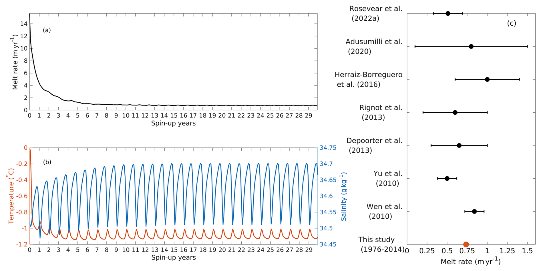
Figure 2 Time series of (a) area-averaged basal melting of AmIS ($\mathrm{m}\cdot {\mathrm{yr}}^{-\mathrm{1}}$), (b) temperature (°C, red line and the y axis on the left) and salinity (g kg⁻¹, blue line and the y axis on the right) in a 30-year spin-up run. (c) Comparisons of the AmIS melt rate among different studies. The black dots represent the estimates of the AmIS melt rates and uncertainties from observational studies. The red dot shows the average of the modelled AmIS melt rate from the Historical simulation (1976–2014) in our study.

Figure 3b–d show the spatial distributions of the AmIS basal melting during the periods of 1976–2014 (Historical) and 2076–2100 under the SSP5-8.5 scenario and the SSP1-2.6 scenario. In general, after the increase in the 2060s, the melting beneath AmIS strongly increases multiple times, and there is almost no refreezing. The time-averaged melt rates over 1976–2014 show that a high melting of ∼ 6 m yr⁻¹ occurs near the grounding line and that most of the ice shelf experiences melting lower than 2 m yr⁻¹ (Fig. 3b). The freezing mainly occurs under the north-western ice shelf, with the highest value of ∼ 1.6 m yr⁻¹ near 69.5° E, −70.5° N (Fig. 3b). Lower freezing rates (<0.2 m yr⁻¹) occur along the ice shelf edges (Fig. 3b). This pattern fits the understanding of the buoyancy-driven meridional overturning circulation, in which warm and dense inflows downwell in the eastern ice shelf cavity while cold and fresh outflows upwell in the western cavity. The time-averaged melt rates during 2075–2100 under SSP5-8.5 show that the melting occupies the entire ice shelf, with the highest melt rates of 42 m yr⁻¹ near the grounding line (Fig. 3c). Most of the areas experience melting between 15 and 35 m yr⁻¹, excluding the north-eastern ice shelf, which exhibits a relatively lower melting of ∼ 5 m yr⁻¹ (Fig. 3c).

The time-averaged melt rates over 2015–2055 under SSP1-2.6 (Fig. 3d) have similar behaviours to those under SSP5-8.5 (Fig. 3c). The spatial distributions of melt rates over 2075–2100 for SSP1-2.6 are similar to those for SSP5-8.5, but with lower melt rates of ∼ 30 m yr⁻¹ near the grounding line and 10–25 m yr⁻¹ over the central and north-western ice shelf (Fig. 3d).

The melt rates in our simulations show higher sensitivity compared with other studies, e.g. Naughten et al. (2018) and Kusahara et al. (2023). This is inherited from the global UKESM1.0-LL model. The model forcing in Naughten et al. (2018) and Kusahara et al. (2023) is taken from ACCESS-1.0 and MIROC-ESM, respectively. Meehl et al. (2020) and Forster et al. (2020) quantified the climate sensitivity of these models and suggested that UKESM1.0-LL has a higher climate sensitivity than the other two models, which might result in a warmer ocean temperature (Sellar et al., 2020). This suggests that our regional model, forced by the outputs from the climate-sensitive UKESM1.0-LL, produces a stronger response to increasing emissions of greenhouse gases.

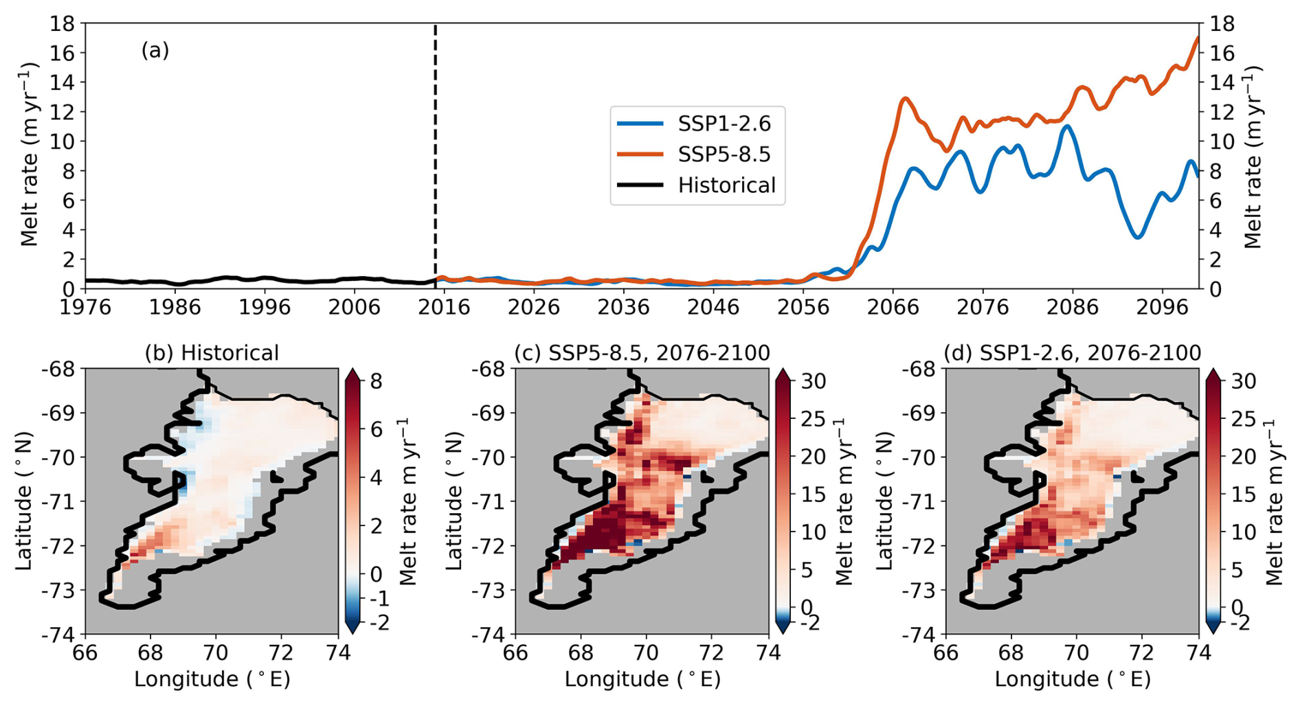
Figure 3 (a) Time series of the area-averaged melt rate (m yr⁻¹) from 1976 to 2100. A 12-month running average is applied. The dashed vertical line indicates the start of 2015. The time-averaged basal melting is shown over the periods (b) 1976–2014 (Historical), (c) 2076–2100 under SSP5-8.5 and (d) 2076–2100 under SSP1-2.6. The warm or cold colours represent melting or refreezing, respectively. Note the different colour map ranges. The colour map for panel (c) is saturated.

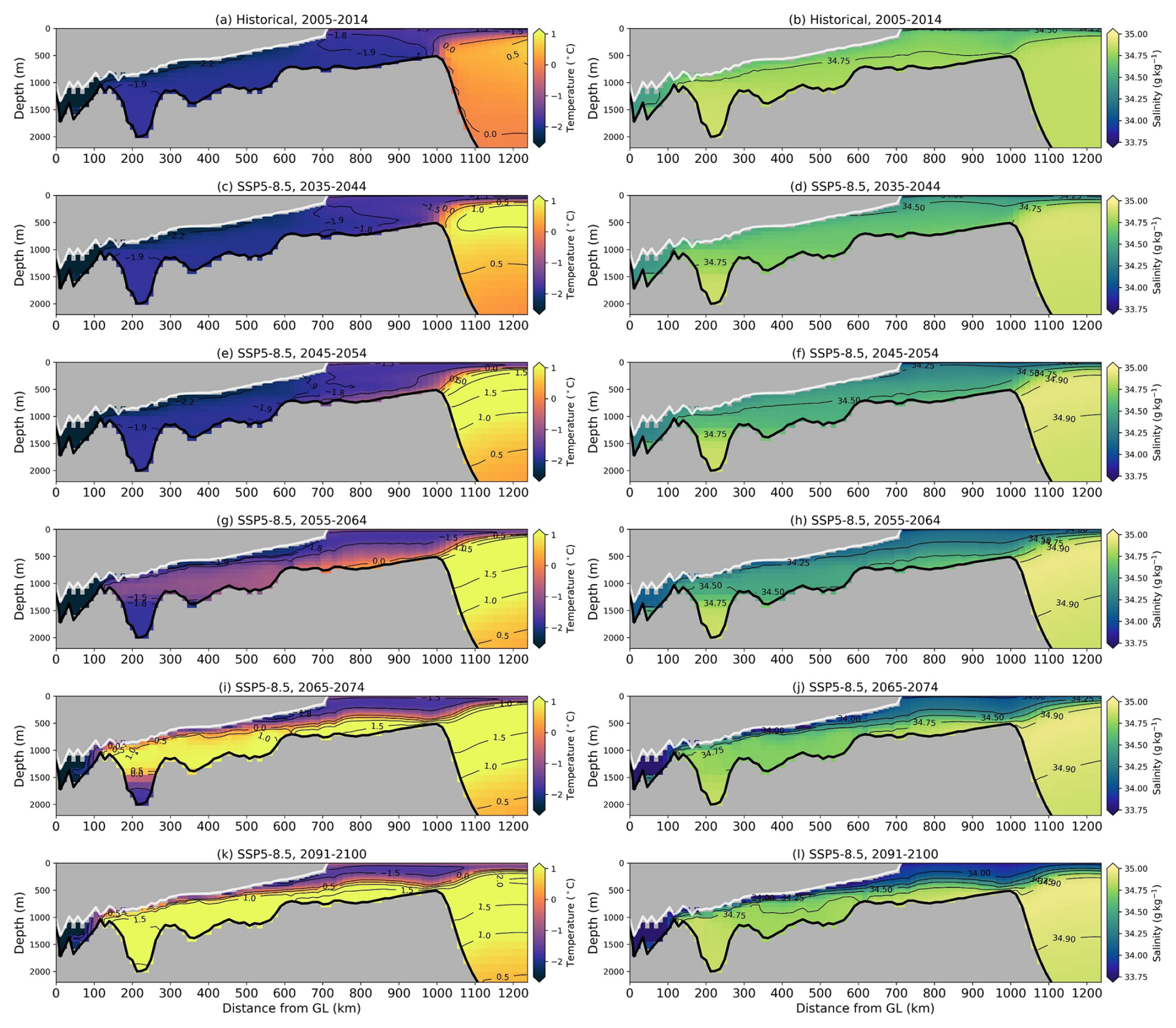
Figure 4 Time mean of temperature and salinity at a transect extending from the grounding line (GL), Prydz Bay Gyre and the shelf break in the SSP5-8.5 scenario. The coordinates show the distance from the GL against the depth below sea level. The location of the transect is shown by the white line in Fig. 1. The years of the time mean are shown in the titles of each panel.

3.1.2 Warming on the continental shelf

For the analyses below, the continental shelf and the shelf sea are defined by the areas between the Antarctic Slope Current and the AmIS calving front or coastal line (Fig. 1). The cavity is defined as the ocean beneath the AmIS draft.

There is a projected warming and freshening on the continental shelf and inside the AmIS cavity. Figure 4 shows temperature and salinity at a transect from the grounding line to the shelf break (the white line in Fig. 1) in the SSP5-8.5 scenario. The warm mCDW off the slope is isolated at the shelf break during the years 2005–2014 (Fig. 4a). The shelf sea is generally below −1.8 °C at depth with a salinity of 34.5–34.75 g kg⁻¹ between 2005 and 2014 (Fig. 4a, b). The cavity temperature is below −1.9 °C, and the salinity in the deeper cavity is higher than 34.75 g kg⁻¹ (Fig. 4a, b). This suggests that the cavity is filled by HSSW between 2005 and 2014. mCDW becomes warmer from the years 2035 to 2044 and penetrates across the shelf break, resulting in an increase in the shelf sea temperature to $<-\mathrm{1.5}$ °C (Fig. 4c). This is accompanied by a decrease in the shelf sea salinity to <34.5 g kg⁻¹ (Fig. 4d). The cavity temperature has little change, with a slight freshening at the shallower depths (Fig. 4c, d). From the years 2045 to 2054, mCDW on the seabed of the shelf sea spreads southward and intrudes into the cavity (Fig. 4e), causing the cavity temperature to increase to ∼ −1.5 °C during the years 2055–2064 (Fig. 4g) and salinity to decrease to 34.25–34.50 g kg⁻¹, except for the deepest cavity (Fig. 4h). This suggests that the dominant water mass in the cavity changes to mCDW between 2055 and 2064, consistent with the abrupt increase in the melt rate in the 2060s. There is further warming in the entire area (Fig. 4i, k). The cavity is flushed by an even warmer mCDW of 0.5–1.5 °C during the years 2091–2100. The enhanced warming and melting of the ice shelf result in strong freshening in the upper cavity and the shelf sea, forming strong stratification at depths of 300–500 m (Fig. 4j, l).

The changes in water masses in the model domain under SSP5-8.5 are illustrated in Fig. 5. The definition of the water masses is given in Table 1. The water mass definitions are primarily based on Galton-Fenzi (2009), with modifications to adapt to our simulations. The plots show temperature against salinity in each grid cell inside the ice shelf cavity (solid dots) and on the continental shelf (open triangles). The black lines show the dilution relation when ice is melted by the warmest water mass in the cavity. During the years 2005–2014, there is a relatively colder mCDW on the continental shelf below 300 m, which might induce the melting of the shallowest ice shelf (Fig. 5a). HSSW occupies the cavity and controls the ice shelf melting at depths below about 800 m (Fig. 5a). ISW clusters at the shallower depth of ∼ 300 m inside the cavity (Fig. 5a). ISW is also found between 800 and 2000 m following the Gade line with the source water of HSSW, suggesting that this is the outflow of meltwater caused by HSSW (Fig. 5a). The temperature of Antarctic Surface Water (AASW) is between −1 and −1.7 °C (Fig. 5a). During the years 2035–2044 and 2045–2054, AASW becomes warmer and more stratified. The temperature of mCDW increases with the increase in the existence of mCDW in the cavity. HSSW still dominates the ice shelf melting (Fig. 5b, c). However, the distributions of HSSW in the entire domain are less. HSSW becomes fresher and is transformed into Low Salinity Shelf Water (Fig. 5b, c). From the years 2055 to 2064, there is little HSSW found within the cavity or on the continental shelf (Fig. 5d–f). mCDW gradually occupies all depths below ∼ 300 m inside and outside the cavity and controls the ice shelf melting (Fig. 5d-f). Less ISW is formed in the shallower cavity, and it becomes fresher, with its potential density decreased from 27.6 to 27.8 kg m⁻³ during the years 2005–2014 to <27.2 kg m⁻³ from the years 2065 to 2074 onwards (Fig. 5d–f). The meltwater on the Gade line, driven by the warm mCDW intruding into the deepest cavity, becomes substantially warm (−2.5–1 °C) with depths from the years 2065 to 2074 (Fig. 5d–f). In addition, the water mass in the shallower cavity (<500 m) is buoyant (26.6–27.8 kg m⁻³). This implies that the warmed and freshened outflow of meltwater increases the buoyancy inside the cavity, enhancing the cavity circulations. AASW becomes warmer and the range of its salinity and density shrinks from the years 2055 to 2064 onwards (Fig. 5d–f), indicating that the stratification at the surface is enhancing.

The evolution of water masses suggests that the AmIS cavity starts to transition from a cold regime to a warm regime in the years 2055–2064 (Fig. 5d) and eventually becomes a warm cavity from the years 2065 to 2074 (Fig. 5e, f).

The time evolution of the depth-mean cavity temperature, salinity, shelf sea temperature and salinity under SSP5-8.5 is shown in Fig. 6. mCDW primarily occupies depths below 300 m in our simulations (Fig. 5), so we choose a depth range of 300 m and below for the shelf sea properties to capture changes in mCDW. Figure 6a shows the time series of temperature. The shelf sea temperature begins to increase from about −1.5 °C in the 2030s to about 0.3 °C in the late 2060s, followed by a slower increase to above 0.5 °C in 2100 (Fig. 6a). By contrast, the cavity temperature is stabilized at about −2 °C before the 2050s and then has an abrupt increase to about 0 °C in the late 2060s and a continuous increase to about 0.4 °C in 2100 (Fig. 6a). The time series of the cavity temperature is consistent with that of the melt rate (Fig. 3a). There is a roughly 20-year delay between the increase in the shelf sea temperature and the increase in the cavity temperature as well as the melt rate. The changes in salinity in the shelf sea salinity and the cavity are similar and more synchronized (Fig. 6b). The two salinities fluctuate between 34.6 and 34.8 g kg⁻¹, start to decrease in the 2030s and then diverge in the 2040s, when the cavity salinity has a larger decrease (Fig. 6b). The difference is likely due to the reduction in sea ice production, which matters in dense water formation, while the increased mCDW is present on the continental shelf but has not yet reached the deeper cavity (Fig. 5b, c). Reduced vertical convection resulting from a more stratified ocean may also cause the difference. Freshwater forcing from ice sheets is prescribed assuming the ice sheet mass is kept constant in UKESM1.0-LL (Sellar et al., 2020), which results in additional snowfall on warmer ice sheets and increased freshwater released at the ocean surface. This bias is propagated through the lateral boundary to the regional domain. The shelf sea salinity and the cavity salinity have a slight bounce in the 2060s and are stable until 2100 (Fig. 6b), suggesting that a denser mCDW occupies the entire domain from the 2060s.

Table 1 Water mass definitions based on temperature (T, °C), salinity (S, g kg⁻¹), potential density (ρ, kg m⁻³) and depth (m) characteristics. T_f is the surface freezing point shown by the dashed line in Fig. 5. AASW: Antarctic Surface Water; mCDW: modified Circumpolar Deep Water; HSSW: High Salinity Shelf Water; LSSW: Low Salinity Shelf Water; ISW: Ice Shelf Water.

The delay of the cavity temperature increase and the larger freshening of the cavity salinity might suggest delayed processes connecting warming on the continental shelf and ice shelf melting, such as the passage of warm water into the cavity.

The projected changes in temperature, salinity and water masses in the SSP1-2.6 scenario have minor differences from those in the SSP5-8.5 scenario (extra figures can be found in Supplement Sect. S2). The delay of the cavity temperature is found in the SSP1-2.6 simulations as well, with a smaller degree of warming and freshening.

Figure 5 Time mean of temperature against salinity diagram for each grid cell within the ice shelf cavity (the solid dots) and on the continental shelf (the open triangles) in the SSP5-8.5 scenario. The grey solid lines are the potential density. The black dashed line shows the surface freezing point. The black solid line represents the Gade line, defined by end-members of the warmest water mass in the cavity (the black pentacle). The colour schemes show the depth of each grid cell. The years of the time mean are shown in the title of each panel.

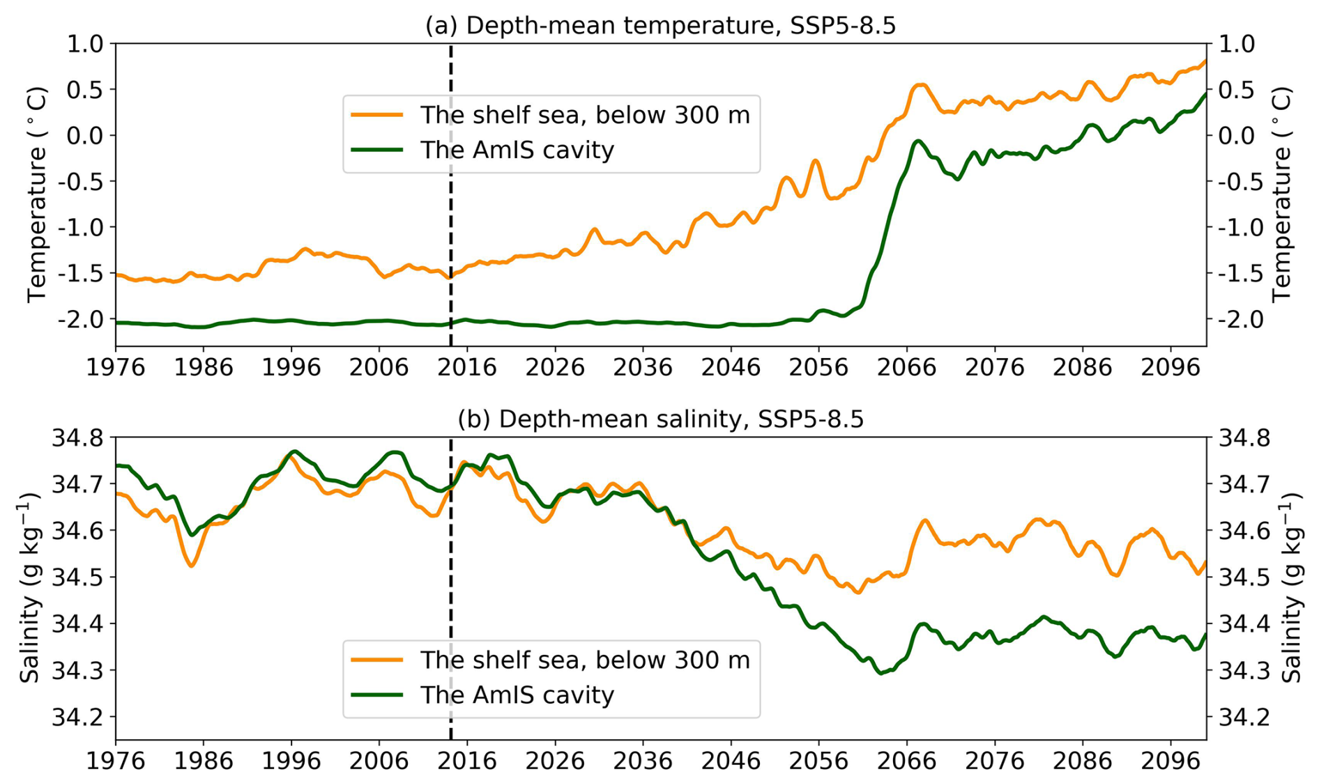
Figure 6 Time series of the depth-mean (a) temperature and (b) salinity averaged within the ice shelf cavity (the green line) and on the continental shelf below 300 m (the orange line) in the SSP5-8.5 scenario. The vertical dashed line indicates the year 2015. A 12-month running average is applied.

3.2 Mechanism causing the delayed increase in AmIS melting

3.2.1 Reversed current-induced increase in heat into the cavity

Figure 7 shows the barotropic streamfunction (BSF) in the model domain in the SSP5-8.5 scenario. As the strength of BSF inside the cavity is much smaller than that outside the cavity, we present them with two different colour schemes. The red–blue colour schemes are for BSF on the open ocean and the orange–purple colour schemes are for BSF in the cavity. The positive or negative BSF represents anti-clockwise or clockwise circulation. The BSF of PBG is positive, suggesting that PBG is anti-clockwise with a strength of ∼ 0.5 Sv and the PBG main flow (indicated by the solid purple line in Fig. 7a) is offshore during the years 2005–2014 (Fig. 7a). The BSF near the AmIS calving front is positive with values of 0.1–0.2 Sv (Fig. 7a), indicating that one of the HSSW inflows is on the western ice shelf front during the years 2005–2024. The BSF in the deeper cavity is negative with values of −0.1 Sv during the years 2005–2024 (Fig. 7a). This suggests that the cavity circulation is clockwise with an HSSW inflow on the eastern ice shelf front. During the years 2035–2044 and 2045–2054, the positive and anti-clockwise PBG is gradually weakened, disappears and transitions to the negative BSF (Fig. 7b, c). This is accompanied by a weakening of the cavity circulation (Figs. 7b, c, 8a), likely due to reduced formation of HSSW outside the AmIS cavity (Fig. 5b, c), which becomes less efficient at driving the cavity circulation. During the years 2055–2064, the negative BSF on the continental shelf is increased (Fig. 7d) and the PBG strength is enhanced (Fig. 8b), although the clockwise PBG has not yet been established (Fig. 7d). The positive cavity BSF near the ice shelf front changes to negative, and the negative BSF in the deeper cavity is increased (Fig. 7d) and the barotropic circulation in the cavity is strengthened during the years 2055–2064 (Fig. 8a). This suggests that the circulations driven by HSSW are very weak or non-existent, and the cavity circulation is controlled by mCDW. From the years 2065–2074, the clockwise PBG is well-established (Fig. 7e, f) and the PBG strength is drastically increased (Fig. 8b). The cavity circulation is greatly strengthened (Figs. 7e, f, 8a).

The evolution of the BSF distribution in the SSP1-2.6 scenario behaves in a similar way to that of the SSP5-8.5 scenario. However, there is a striking difference in that the PBG and the cavity circulation strength decline in the 2090s in SSP1-2.6 but not in SSP5-8.5 (Fig. 8). The decline is consistent with the decrease in the melt rate in the 2090s in the SSP1-2.6 scenario. We will discuss these variations in Sect. 3.2.2.

To understand the changes in the relationship between ice shelf melting and ocean circulations inside and outside the cavity, we calculated the heat budget in the cavity as in Jourdain et al. (2017). Neglecting diffusion in ice and the interior ocean, the heat flux entering the ice cavity (H_in) is simplified into three components: the heat used to melt the ice shelf (H_lat), the heat that warms or cools the seawater within the cavity (H_{HC_VAR}) and the remaining heat flux that exits the cavity (H_out):

$$\begin{array}{}\text{(1)}& {\displaystyle }{H}_{\mathrm{in}}=H_{\mathrm{out}}+H_{\mathrm{lat}}+H_{\mathrm{HC}\mathrm{\_}\mathrm{VAR}},\text{(2)}& {\displaystyle }{H}_{\mathrm{in}}={\mathit{\rho }}_{\mathrm{ref}}{C}_p\underset{r\in \mathrm{front},u>\mathrm{0}}{\iint }u(r,z)\left(T\right(r,z)-T_f^{\mathrm{0}})\mathrm{d}r\mathrm{d}z,\text{(3)}& {\displaystyle }{H}_{\mathrm{out}}={\mathit{\rho }}_{\mathrm{ref}}{C}_p\underset{r\in \mathrm{front},u<\mathrm{0}}{\iint }u(r,z)\left(T\right(r,z)-T_{\mathrm{f}}^{\mathrm{0}})\mathrm{d}r\mathrm{d}z,\text{(4)}& {\displaystyle }{H}_{\mathrm{lat}}=L_f\underset{x,y\in \mathrm{draft}}{\iint }{\mathit{\rho }}_{i}m\mathrm{d}x\mathrm{d}y,\text{(5)}& {\displaystyle }{H}_{\mathrm{HC}\mathrm{\_}\mathrm{VAR}}={\mathit{\rho }}_{\mathrm{ref}}{C}_p\underset{x,y,z\in \mathrm{cavity}}{\iint }{\displaystyle \frac{\mathrm{d}T(x,y,z)}{\mathrm{d}t}}\mathrm{d}x\mathrm{d}y\mathrm{d}z.\end{array}$$

ρ_ref is the reference seawater density of 1026 kg m⁻³, C_p is the specific heat capacity of 3991.87 J K⁻¹ kg⁻¹, and u(r,z) is the velocity perpendicular to the ice shelf front (positive into the ice shelf cavity). T(r,z) is the temperature along the ice shelf front. $T_{\mathrm{f}}^{\mathrm{0}}$ is the surface freezing point. L_f equal to 334 J kg⁻¹ is the latent heat of fusion of ice. ρ_im is the melt rate (kg m⁻² s⁻¹). The latent heat of the ice shelf (H_lat) is obtained from the model outputs. $\mathrm{d}T(x,y,z)$ is the temperature change in the same grid cell. dt is 1 month. The variables used in the calculations are monthly mean model outputs.

Figure 9 shows the time evolution of the heat budget in the cavity in the SSP5-8.5 and SSP1-2.6 scenarios. H_in starts to increase in about the 2040s and abruptly increases in the 2060s in two scenarios. This is consistent with the water mass changes in the cavity (Fig. 5) and the development of the BSF of PBG (Fig. 7). H_{HC_VAR} is at least 1 order of magnitude smaller than H_lat and H_out. The increase in H_lat begins in the 2060s, and its behaviours are similar to the changes in the strength of the cavity circulation and PBG. This might suggest that the increased ice shelf melting enhances the barotropic flow inside the cavity and in front of the ice shelf, as stronger pressure or density gradients are created (Jenkins, 2016; Jourdain et al., 2017). The melt rate-circulation strength coherence is similar to the melt-induced circulation found in the Jourdain et al. (2017) Amundsen Sea study. H_out follows and is comparable to H_lat, suggesting that about 50 % of heat is unused and leaves the cavity.

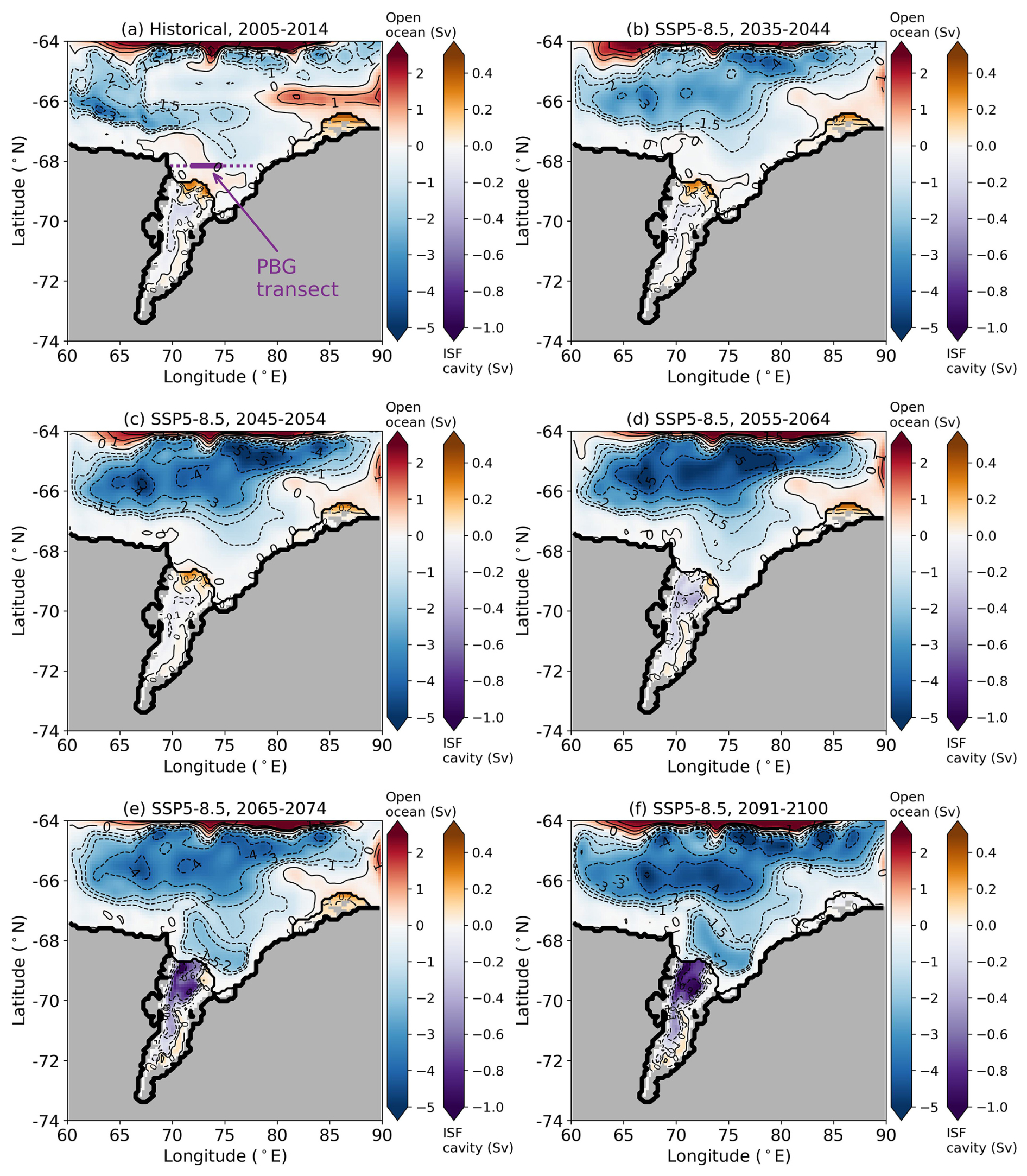
Figure 7 Time mean of the barotropic streamfunction (BSF, Sv) in the SSP5-8.5 scenario. The red–blue colour schemes are for BSF in the open ocean. The values of the BSF contours in the open ocean are −5, −4, −3, −2, −1.5, −1, 0, 1, 1.5 and 2 Sv. The orange–purple colour schemes are for BSF in the ice shelf cavities. The values of the BSF contours in the cavities are −0.9, −0.6, −0.3, −0.1, 0, 0.1 and 0.2 Sv. The positive or negative BSF represents anti-clockwise or clockwise circulation. The solid and dotted purple lines show the PBG transect and the extended transects to the coasts. The years of the time mean are shown in the title of each panel.

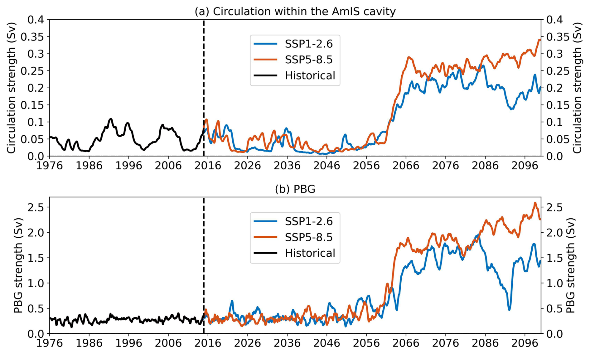
Figure 8 Time series of (a) the strength of the barotropic cavity circulation and (b) the strength of PBG. The strength of the cavity circulation and PBG is defined as the absolute value of the area-mean BSF. The PBG area is defined using the closed BSF contour of −1.5 Sv in front of the ice shelf in Fig. 7f. The vertical dashed line indicates the year 2015. A 12-month running average is applied.

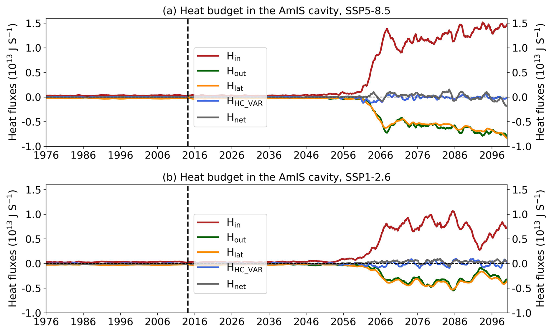
Figure 9 The heat budget of the ice shelf cavity for (a) the SSP5-8.5 scenario and (b) the SSP1-2.6 scenario. The heat of the ice shelf cavity system comprises the heat flux into the cavity (H_in, the red line), the heat used to melt ice or the latent heat of ice (H_lat, the orange line), the heat exiting the cavity (H_out, the green line) and the heat used to warm or cool the seawater in the cavity (H_{HC_VAR}, the navy line). The net heat flux (H_net) is equal to $H_{\mathrm{in}}-(H_{\mathrm{lat}}+H_{\mathrm{out}}+H_{\mathrm{HC}\mathrm{\_}\mathrm{VAR}}$). The vertical dashed line indicates the year 2015. A 12-month running average is applied.

The changes in ocean circulations and heat fluxes in the cavity explain the question posed above. Why does the abrupt increase in the melt rate start ∼ 20 years later than the increase in the shelf sea temperature? PBG is anti-clockwise and weak before the 2050s, with off-shore transport at the PBG transect (Fig. 7a–c). Despite the warming and increased mCDW on the continental shelf (Figs. 4a, c, e, 5a–c), the processes of mCDW intruding into the cavity are slow before the 2060s (Figs. 8b, 9). An effective pathway of mCDW into the cavity starts to be established in the years 2055–2064 (Fig. 7d), and the clockwise PBG is well established and sustained from the years 2065–2074 (Figs. 7e, f, 8b), which transports massive heat into the cavity (Fig. 9) and transforms the cavity into a warm regime (Fig. 5e), resulting in the abrupt increase in the melt rate after the 2060s (Fig. 9).

3.2.2 Freshening-driven reversed current

The previous section demonstrated that the reversal of the PBG main flow allows the increasing oceanic heat to penetrate the AmIS cavity, causing increased basal melting. We will now discuss what causes the PBG to reverse. The following analysis does not qualitatively vary between SSP5-8.5 and SSP1-2.6, so we only present the results from SSP5-8.5 here.

Here, we focus on a zonal section of PBG at Amery Depression (solid purple line in Fig. 7a) and its extensions to the western and eastern banks (dotted purple lines in Fig. 7a). The area between the vertical dashed purple lines represents the PBG transect. Figure 10a shows that warming in the east of PBG begins in the 2040s and gradually spreads westward across PBG until the mid-2060s, when a sharp increase in temperature occurs. The temperature west of PBG is always cooler due to the injections of the cold outflow of meltwater (Fig. 10a). The salinity exhibits notable changes (Fig. 10b). There is a higher salinity and potential density in PBG and its western regions than in the east before the 2040s. Then the entire section has a decline in salinity until the mid-2060s, when the west of PBG experiences a sudden freshening, while PBG and its eastern section have an increase in salinity and potential density. This results in a reversed horizontal salinity and density gradient at the western boundary of PBG. Afterwards, the reversed gradient is sustained. As suggested in Jenkins (2016) and Jourdain et al. (2017), the changes in the barotropic coastal current induced by ice shelf melting can be a geostrophic adjustment due to the changes in pressure gradients. Here we present the sea surface height (SSH) gradient in Fig. 10c. The SSH gradient mirrors salinity and density changes (Fig. 10c). The positive or negative SSH gradient indicates that the SSH in the east is higher or lower than in the west. The SSH gradient is positive in PBG before the 2040s, suggesting that there is a high SSH. The SSH gradient exhibits more fluctuations between the 2040s and 2060s, and a reversed SSH gradient in the west follows the density variations. This suggests that the outflow of AmIS meltwater may have a large impact on the local SSH gradients. The BSF in the section tells a similar story where PBG is positive and anti-clockwise until it completely reverses in the mid-2060s (Fig. 10d).

Figure 11 shows time series of the main surface forcing in the SSP5-8.5 scenario. Freshwater flux from ice shelf melting exhibits the same behaviours as the properties we analysed above (Fig. 11a). The net sea ice production over the continental shelf shows a decrease from the 2040s (Fig. 11b), which might be the source of the freshening of the PBG and the extended section in the 2040s (Fig. 10b). The zonal and meridional surface stress at the ocean surface (from wind or sea ice) does not behave in a similar way to the BSF of PBG (Fig. 10c, d). The southward Ekman transport in the PBG section remains at a magnitude of 0.2–0.3 Sv throughout the simulation. This is much smaller than the mean BSF of the reversed PBG, which increases from 0.5 Sv in the 2060s to over 2 Sv thereafter (Fig. 8). This suggests that surface stress is not a direct factor in the PBG reversal. The geostrophic component is probably more influential. However, Ekman pumping (calculated from the surface stresses at the ocean surface) in the PBG area, which strengthens the upwelling of mCDW onto the continental shelf (Greene et al., 2017), is enhanced between the 2040s and 2070s, with large fluctuations afterwards (Fig. 11e). The increased Ekman pumping coincides with the increased temperature in the PBG section (Fig. 10a) and the reduction in sea ice production from the 2040s (Fig. 11b). Figure 11 suggests that the enhanced Ekman pumping in the 2040s might be responsible for the freshening in the PBG section and the unstable PBG between the 2040s and 2060s, and the abruptly increased ice shelf melting further develops and sustains the reversed salinity or density gradient between PBG and its western regions. The Ekman pumping may also contribute to the changes in the local SSH gradients in the 2060s (Fig. 10c).

Figure 10 Hovmöller diagram of properties at the zonal transect shown in Fig. 7a. (a) Depth-mean temperature below 300 m. (b) Depth-mean salinity below 300 m. The potential density below 300 m overlies the temperature and salinity. The values of the potential density contours are 27.3, 27.4, 27.5, 27.6, 27.7 and 27.8 kg m⁻³. (c) Zonal sea surface height gradient (SSH gradient). A positive or negative SSH gradient indicates that the SSH in the east is higher or lower than in the west. The values of the SSH gradient contours are −3, −2.5, −1.5, −0.5, 0, 0.25, 1 and 2 mm km⁻¹. (d) Barotropic streamfunction (BSF). The values of the BSF contours are −2.5, −2, −1.5, −1, −0.5, 0, 0.25, 0.5 and 1 Sv. A positive or negative BSF represents anti-clockwise or clockwise circulation. The transect between the purple dashed lines is the PBG transect shown by the solid purple line in Fig. 7a. A 12-month running average is applied.

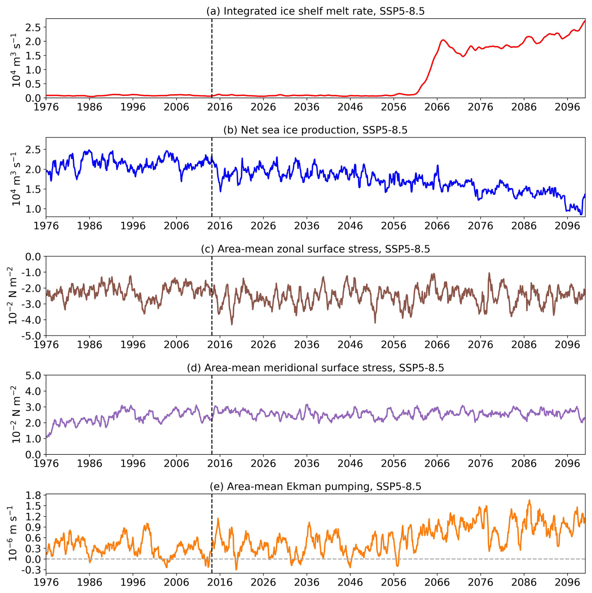
Figure 11 Time series of (a) integrated ice shelf freshwater fluxes (10⁴ m³ s⁻¹), (b) net sea ice production over the continental shelf (10⁴ m³ s⁻¹), (c) area-mean zonal surface stress within the PBG area (10⁻² N m⁻²), (d) area-mean meridional surface stress within the PBG area (10⁻² N m⁻²) and (e) area-mean Ekman pumping within the PBG area (10⁻⁶ m s⁻¹) in the SSP5-8.5 scenario. The surface stress refers to the stress on the ocean surface (i.e. from either wind or sea ice). Ekman pumping is calculated based on the surface stresses. The PBG area is defined using the closed BSF contour of −1.5 Sv in front of the ice shelf in Fig. 7f. The vertical dashed line indicates the year 2015. A 12-month running average is applied.

Figures 10 and 11 suggest that the reversal of PBG is controlled by the stronger freshening west of PBG due to the outflow of ice shelf meltwater, which caused a reversed density distribution and SSH gradient. PBG is reversed due to the adjustment of the new pressure gradient. Here we present a simple scale analysis of the meridional current. As the contribution from the surface stress τ_x is small (Fig. 11c), the meridional current can be expressed as

$$\begin{array}{}\text{(6)}& fv={\displaystyle \frac{\mathrm{1}}{{\mathit{\rho }}_{\mathrm{ref}}}}{\displaystyle \frac{\mathrm{d}p}{\mathrm{d}x}},\end{array}$$

where $f=-\mathrm{1.4}$ × 10⁻⁴ s⁻¹ is the Coriolis parameter, v is the time-averaged meridional velocity, ρ_ref=1026 kg m⁻³ is the reference seawater density and dx is the horizontal grid spacing. dp is the horizontal pressure difference. Using the hydrostatic hypothesis,

$$\begin{array}{}\text{(7)}& \mathrm{d}p=gH\mathrm{d}\mathit{\rho }+g{\mathit{\rho }}_{\mathrm{ref}}\mathrm{dSSH},\end{array}$$

g=9.81 m s⁻² is gravity and H≈600 m is the depth to the seabed. dSSH is the horizontal difference of the sea surface height. Using a linear equation of state, and assuming that the temperature difference does not produce a significant change in density (Fig. 10a),

$$\begin{array}{}\text{(8)}& \mathrm{d}\mathit{\rho }=b\mathrm{d}S,\end{array}$$

with b=0.78 kg m⁻³, dS is the spatial salinity difference between PBG and its western regions. Therefore, the meridional velocity can be attributed to the effect of the salinity gradient and sea surface height gradient:

$$\begin{array}{}\text{(9)}& v={\displaystyle \frac{g}{f}}\left({\displaystyle \frac{Hb}{{\mathit{\rho }}_{\mathrm{ref}}}}{\displaystyle \frac{\mathrm{d}S}{\mathrm{d}x}}+{\displaystyle \frac{\mathrm{dSSH}}{\mathrm{d}x}}\right).\end{array}$$

The estimates are shown in Fig. A1. The term of salinity gradient ($\frac{Hb}{{\mathit{\rho }}_{\mathrm{ref}}}\frac{\mathrm{d}S}{\mathrm{d}x}$) has a magnitude of 8 × 10⁻⁶ (Fig. A1a). The magnitude of the horizontal SSH gradient ($\frac{\mathrm{dSSH}}{\mathrm{d}x}$) is up to 4 × 10⁻⁶ (Fig. A1b), which is less than 50 % of the salinity effect. The reconstructed meridional velocity based on Eq. (9) agrees with the modelled velocity (Fig. A1c). This analysis suggests that the effect of salinity gradient and SSH gradient compete (Fig. A1a, b). However, the reversal of PBG is a consequence of the reversal of horizontal salinity differences between PBG and its western regions.

The reversal of PBG is also documented by Galton-Fenzi (2009). In his study, the clockwise PBG does not exist in winter because dense water formed in the Barrier Polynya blocks the current from the Prydz Bay Channel and prevents mCDW from accessing the ice shelf cavity (Galton-Fenzi, 2009). When the Barrier Polynya is active, the clockwise PBG is dumped (Galton-Fenzi, 2009). In our simulation, the seasonality of the PBG reversal is weaker than that in Galton-Fenzi (2009) (Fig. 10d). This is due to the overestimated sea ice concentration (SIC) in the Barrier Polynya region (the white dashed box in Fig. 12a) in our simulation (Fig. 12), which is inherited from the overestimation of the summer SIC in the model forcing taken from the UKESM1.0-LL outputs (Roach et al., 2020). The modelled climatological summer SIC in the Barrier Polynya between 1978 and 2014 is 50 %–60 % (Fig. 12a), while the observed SIC in the Barrier Polynya is up to 20 %, with 30 %–50 % SIC in the upstream regions (Fig. 12b). Our model failed to capture the spatial features. The seasonal climatology of SIC in the Barrier Polynya during the historical period shows that the modelled SIC in December, January and February is at least twice as high as the observations (Fig. 12c). It also overestimates the SIC in other months. However, the SIC after December decreased drastically in the two SSP scenarios, and the January, February and March SIC values are below 20 % (Fig. 12c). This indicates that the overestimated SIC in the Barrier Polynya weakens the seasonal reversal of PBG in our simulations. In addition, this suggests that the overestimated sea ice mitigates the warm intrusions onto the shelf sea as the clockwise PBG is hard to establish well in summer. The reduction in sea ice production in the 2040s (Fig. 11b) opens a wider gate to the formation of the clockwise PBG. Although sea ice in front of the ice shelf is not the direct trigger for the reversal of PBG in the 2060s, it establishes the necessary pre-conditions for this event. This implies that a decrease in sea ice production in Prydz Bay could serve as a climate indicator of the increasing AmIS basal melt. Direct observation of ice shelf basal melting is challenging, but long-term sea ice records exist. A decreasing trend of sea ice may signal a forthcoming increase in basal melt rates.

The mechanism, in which the stronger freshening at the ice shelf front drives the reversal of PBG main flow, is valid in the SSP1-2.6 scenario as well (Fig. A2). The reduced sea ice in the Barrier Polynya opens the channel and enables the establishment of the clockwise PBG. This mechanism is self-maintained: the warm water flushes the sub-ice shelf cavity, and the strengthened outflow of ice shelf meltwater reverses the salinity–density differences and stabilizes the clockwise gyre. The southward main flow will carry more warm water to the cavity and sustain the feedback loop.

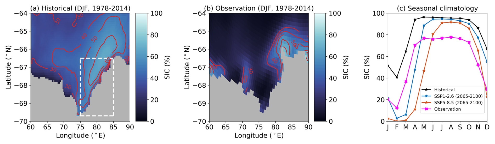
Figure 12 Time-mean summer (DJF) sea ice concentration (SIC) between 1978 and 2014 from (a) the historical simulation in this study (Historical) and (b) observations. The observation dataset is Sea Ice Concentrations from Nimbus-7 SMMR and DMSP SSM/I-SSMIS Passive Microwave Data published by the National Snow and Ice Data Center (NSIDC). The white dashed box in panel (a) shows the location of the Barrier Polynya. (c) Seasonal climatology of SIC within the Barrier Polynya. The seasonal climatology of the two SSP scenarios is calculated between 2065 and 2100.

This leads to a remaining question: what causes the decline in the melt rate (Fig. 3a) and the associated weakening of PBG (Fig. 8b) in the 2090s in the SSP1-2.6 scenario? This is controlled by the variability of the shelf sea temperature on the upstream ocean boundary. Figure A3 shows time series of temperature and salinity on the continental shelf in the upstream boundary. There is a warming from 2015 to the 2040s–2050s and temperature plateaus afterwards (Fig. A3a). This trend has good agreement with the shelf sea temperature changes (Fig. 6a) and melt rate evolution (Fig. 3a). This suggests that the local warming and freshening near the ice shelf front ultimately come from the upstream ocean boundary. In addition, there is a decrease in the shelf sea temperature on the upstream boundary from ∼ 1.25 to 0.75 °C in the 2090s under SSP1-2.6. This decline in temperature forcing results in the decrease in melt rate under SSP1-2.6 (Fig. A3a) and a transient recovery of PBG (Fig. A2d) in the 2090s. This implies that the gyre reversal is not irreversible. A decrease in temperature could stop this mechanism.

To validate the robustness of the freshening-driven mechanism, we conducted a second series of simulations with forcings taken from the r2 member of the UKESM1.0-LL ensemble. We chose the r2 member as its mid-depth temperature in the SSP1-2.6 scenario within the entire domain starts to increase ∼ 20 years later than that in the r1 member (Fig. S7c). The melt rate jump and PBG reversal in the SSP1-2.6 scenario also exhibit a delay compared to the r1 simulations (Fig. S8–10). A more detailed description of the r2 experiments can be found in Supplement Sect. S3. The differences between the r1 and r2 series of experiments highlight the importance of ocean boundary conditions, especially the variability of temperature forcing, to the ice shelf melt rate in our regional configuration.

4 Conclusions and discussions

This study investigates the future changes in the AmIS–PB system in the SSP5-8.5 and SSP1-2.6 scenarios. An abrupt increase in AmIS basal melting is projected to happen in the 2060s in both scenarios. The area-averaged melt rate of AmIS is projected to increase from 0.75 ± 0.15 m yr⁻¹ over the period 1976–2014 to 8.10 ± 1.53 m yr⁻¹ over the period 2076–2100 under SSP1-2.6 and to 13.14 ± 2.36 m yr⁻¹ over the period 2076–2100 under SSP5-8.5. The time-mean melt rates during 2076–2100 (when it is in the high melting state) under both SSP1-2.6 and SSP5-8.5 display no refreezing beneath AmIS, and the melting at the grounding line exceeds 30 m yr⁻¹. Drastic warming on the continental shelf and in the AmIS cavity causes increased basal melting. However, the increase in temperature on the continental shelf is in the late 2030s, which happens ∼ 20 years before the jump in AmIS basal melting in the 2060s. The delayed increase in the AmIS melt rate is due to the reversal of the PBG main flow.

PBG plays an important role in the changes in the basal melt of AmIS. The clockwise PBG is not well established due to the sea ice in the active Barrier Polynya, which obstructs its formation. The main flow is northward before about the 2060s, preventing the increased mCDW from intruding into the AmIS cavity and delaying the increase in AmIS melting. However, the main flow of PBG reverses southward after the 2060s as the clockwise PBG is well established. The southward main flow imports substantial mCDW into the cavity, which leads to the increase in AmIS melting. The changes in PBG are due to (1) the reduction in sea ice in the 2030s–2040s, which allows the establishment of the clockwise PBG, and (2) the reversal of the horizontal salinity (and then density) differences between Amery Depression and its western regions. The redistribution of the salinity gradients is established by the strengthened outflow from the AmIS cavity after the 2060s.

A similar mechanism for the regime change is found on the Filchner–Ronne Ice Shelf (Hellmer et al., 2012, 2017; Naughten et al., 2021; Siahaan et al., 2022) and Ross Ice Shelf (Siahaan et al., 2022). A redirection of coastal currents is driven by a reversed density gradient across the Filchner Trough (Hellmer et al., 2012, 2017; Naughten et al., 2021; Siahaan et al., 2022) and Little America Basin in the Ross Sea (Siahaan et al., 2022), which facilitates the penetration of mCDW into the ice shelf cavity and causes the regime change. The similar processes found in the sectors for the three large cold ice shelves emphasize the importance of buoyancy changes in the shelf sea in a warming future. This suggests the necessity of long-term records for the shelf sea salinity and sea ice in order to obtain an early warning of the regime change in the three large cold cavities.

Most cold ice shelf sectors have a structure with steep isopycnals at the continental shelf break (Thompson et al., 2018). The coastal geostrophic flow along the isopycnals is sensitive to the structural changes (Thompson et al., 2018). In this study, we only focus on the interactions between AmIS melting and local circulation. However, there remain many open questions for future studies. For example, how does the geostrophic flow respond to different components of freshwater fluxes from ice shelves, sea ice, icebergs, advections and precipitations? What is the role ocean currents play in connecting the future changes in the freshwater components? What is the threshold of freshening on the continental shelf for the redirected or reversed current? Does the threshold vary between the different shelf sea sectors? A series of freshwater perturbation experiments across various climate scenarios would help address these questions.

Quantifying the future stability of AmIS and its upstream ice sheets is beyond our research scope, but this study can provide implications to some extent. Two previous ice sheet modelling studies (Pittard et al., 2017; Gong et al., 2014) conducted similar extreme experiments by applying enhanced basal melting of AmIS. Both studies suggested that only the collapse of almost the entire ice shelf by unrealistically high basal melting causes the grounding line to retreat beyond the topographic sill. Excluding the most extreme climate scenarios, AmIS is attributed to sea level fall (Gong et al., 2014; Pittard et al., 2017). The stability of AmIS and the upstream ice sheets is primarily buttressed by the topographic sill tens of kilometres upstream of the grounding line (Gong et al., 2014; Pittard et al., 2017). In our SSP5-8.5 simulation, the basal melt rate is not as high as that applied in the extreme experiments in Pittard et al. (2017), with >50 and 100 m yr⁻¹ for two extreme scenarios. It is reasonable to consider that AmIS will remain stable in the next century. However, the high basal melting puts the AmIS at risk of instability in the longer-term warming future. Coupling our stand-alone ocean configuration with an ice sheet model will be a future step in addressing the question of AmIS stability.

We note that the basal melting in this study might be overestimated. In the AME025 configuration, we use the velocity-dependent “three-equation” parameterization of ice–ocean thermodynamics (Jenkins et al., 2010). This parameterization assumes that ice shelf melting is driven by turbulent mixing due to shear currents. However, the turbulent processes at the ice shelf–ocean interface can also be produced by the convection due to buoyancy forcing (Wells and Worster, 2008). For an ice shelf with a stable stratification at the ice shelf–ocean interface, such as AmIS (Rosevear et al., 2022b), the velocity-dependent three-equation parameterization may overestimate basal melting of AmIS (Rosevear et al., 2022a). This results in the projected melt rate likely being overestimated. In addition, UKESM1.0-LL has a higher climate sensitivity compared with other CMIP6 models (Meehl et al., 2020; Forster et al., 2020) and previous generations of climate models (Sellar et al., 2020). This might produce an overestimated and more rapid warming in our regional projections compared with other studies (Naughten et al., 2018). Moreover, we do not include the frazil processes in this configuration. Galton-Fenzi et al. (2012) suggested that the inclusion of frazil in the AmIS simulation decreases the melt rates and increases the arrection rates. No frazil ice in our simulation may result in overestimation. Another source of overestimation is the static ice shelf draft. The ice shelf melt rate is not only temperature-dependent (Holland et al., 2008; Xu et al., 2013) but also basal-slope-dependent (Payne et al., 2007; Little et al., 2009; Magorrian and Wells, 2016). Steeper slopes might increase the heat entrained into the ice shelf and drive higher melting (Payne et al., 2007; Little et al., 2009; Magorrian and Wells, 2016). When AmIS is thinning, it will become smoother and flatter, and the melt rate is expected to be to some extent decreased. Given the limited grounding line retreat of AmIS (Gong et al., 2014; Pittard et al., 2017), which feeds limited deep and steep grounded ice to the floating AmIS, the basal melting beneath the majority of AmIS north of the grounding line may be overestimated. Another limitation is that, due to the relatively coarse grid spacing of ∼ 7–12 km for our model configuration relative to the estimated Rossby radius of 3 km over Prydz Bay (Liu et al., 2017), we cannot investigate the effect of mesoscale eddies on the AmIS basal melting. Liu et al. (2017) suggested that 52 % of the total onshore heat transport across a zonal transect (73–78° E, 67.5° S) in the AmIS front is induced by mesoscale eddies. Given the importance of the mesoscale eddy for warm intrusion beneath Antarctic ice shelves (St-Laurent et al., 2013; Thompson et al., 2018; Stewart et al., 2018, 2019), it is worth employing a higher-resolution model (∼ 1 km) to understand how mesoscale eddies impact future ice shelf melting.

The basal melt rate is projected to exceed 15 m yr⁻¹ beneath the majority of the AmIS after the abrupt increase in both scenarios (Fig. 3c, d). The thinning of the ice shelf results in many changes, e.g. the geometry of the ice shelf cavity or the increased water column thickness under the ice shelf. This is related to a scientific question: how does the time-varying ice shelf draft modify ocean circulations in the cavity and ice shelf–ocean interactions in model simulations? Holland et al. (2023) suggests that a time-varying ice geometry of Thwaites Glacier leads to an increase in melting by more than 30 %, without any change in ocean forcing. However, we use a static ice shelf draft in the AME025 configuration, which limits the ability to investigate such geometrical feedback. Future work would greatly benefit from the development of two-way coupled ocean–ice sheet models and more sophisticated Earth system models (Jordan et al., 2018; Smith et al., 2021; Siahaan et al., 2022; De Rydt and Naughten, 2023).

Appendix A: Extra figures

A1 The effect of the salinity gradient and SSH gradient on PBG

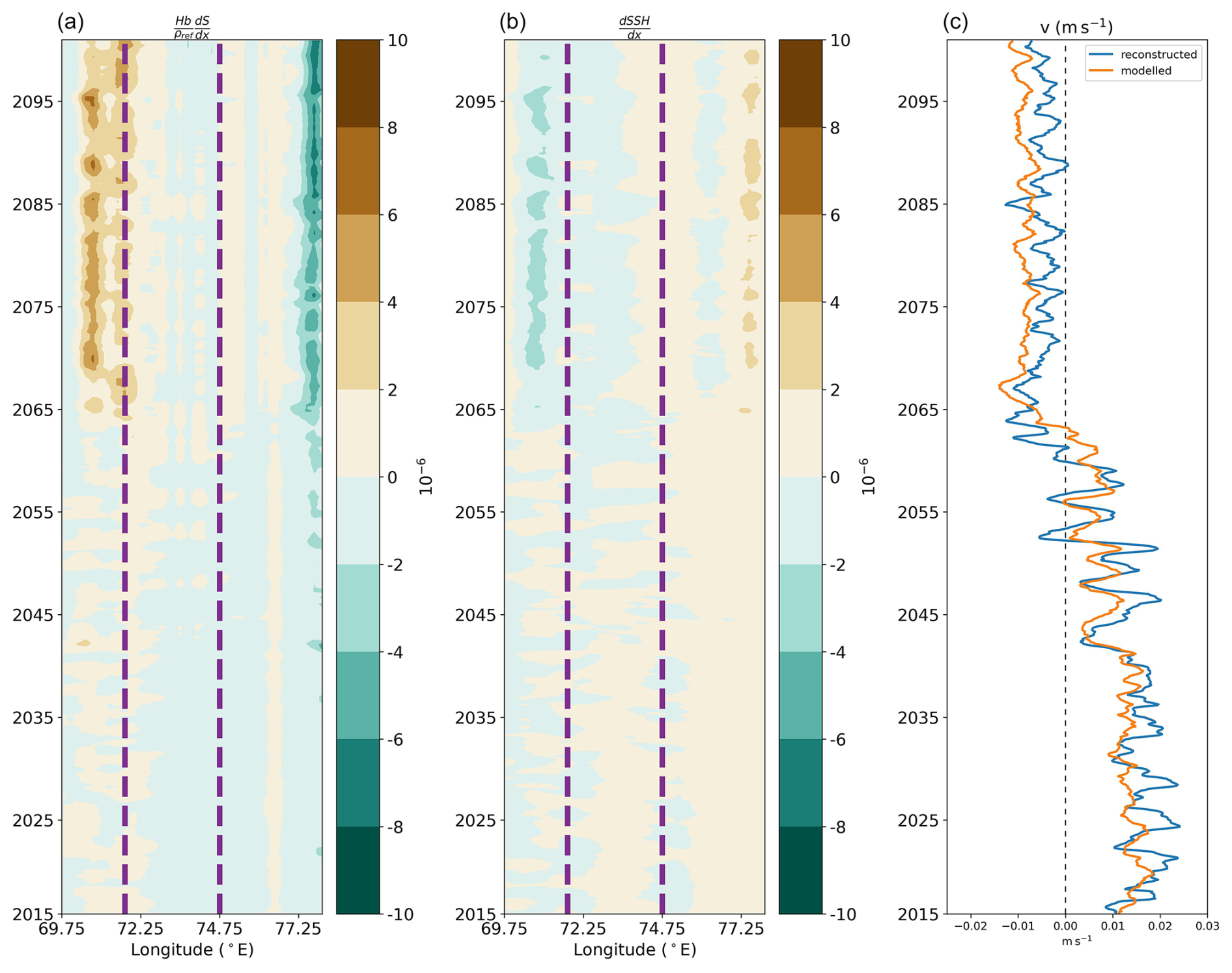
Figure A1 Hovmöller diagram of properties at the zonal transect shown in Fig. 7a in the SSP-5.8 scenario for (a) the salinity gradient term and (b) the sea surface height (SSH) gradient. A positive or negative salinity or SSH gradient indicates that the salinity or SSH in the east is higher or lower than in the west. (c) Time series of the averaged meridional velocity between the two dashed lines. The blue line shows the reconstructed velocity from Eq. (9), and the orange line represents the modelled velocity. A 12-month running average is applied.

A2 Extra figures for the SSP1-2.6 experiment

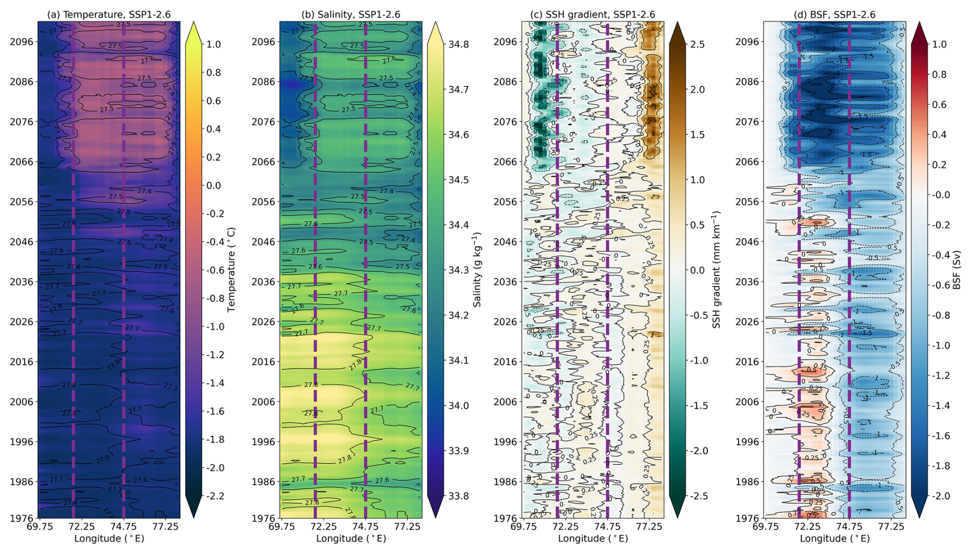
Figure A2 Hovmöller diagram of properties at the zonal transect shown in Fig. 7a. (a) Depth-mean temperature below 300 m. (b) Depth-mean salinity below 300 m. The potential density below 300 m overlies the temperature and salinity. The values of the potential density contours are 27.3, 27.4, 27.5, 27.6, 27.7 and 27.8 kg m⁻³. (c) Zonal SSH gradient. A positive or negative SSH gradient indicates that the SSH in the east is higher or lower than in the west. The values of the SSH gradient contours are −3, −2.5, −1.5, −0.5, 0, 0.25, 1 and 2 mm km⁻¹. (d) Barotropic streamfunction (BSF). The values of the BSF contours are −2.5, −2, −1.5, −1, −0.5, 0, 0.25, 0.5 and 1 Sv. A positive or negative BSF represents anti-clockwise or clockwise circulation. The transect between the purple dashed lines is the PBG transect shown by the solid purple line in Fig. 7a. A 12-month running average is applied.

A3 The forcing of temperature and salinity at the upstream ocean boundary

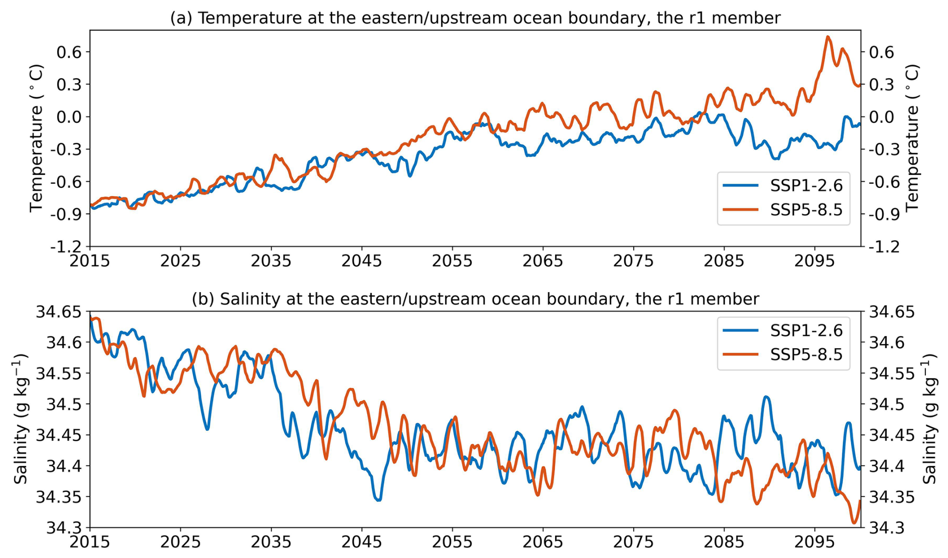
Figure A3 (a) Time series of the area-averaged temperature of ocean boundary forcing at the upstream boundary from 2015 to 2100. A 12-month running average is applied. (b) The same but for salinity ocean boundary forcing.