Ice sheet model simulations reveal that polythermal ice conditions existed across the northeastern USA during the Last Glacial Maximum

Geologic archives of the Laurentide Ice Sheet (LIS) provide abundant constraints regarding the size and extent of the ice sheet during the Last Glacial Maximum (LGM) and throughout the deglaciation. Direct observations of LGM LIS thickness are non-existent, however, due to ice surface elevations likely exceeding those of even the tallest summits in the northeastern United States (NE USA). Geomorphic and isotopic data from mountains across the NE USA can inform basal conditions, including the presence of warm- or cold-based regimes, while covered by ice. While warm-based ice and erosive conditions likely existed on the flanks of these summits and throughout neighboring valleys, cosmogenic nuclide inheritance and frost-riven blockfields on summits suggest ineffective glacial erosion and cold-based ice conditions. Geologic reconstructions indicate that a complex erosional and thermal regime likely existed across the NE USA sometime during and after the LGM, although this has not been confirmed by ice sheet models. Instead, current ice sheet models simulate warm-based ice conditions across this region, with disagreement likely arising from the use of low-resolution meshes (e.g., > 20 km) which are unable to resolve the high bedrock relief across the NE USA that strongly influenced overall ice flow and the complex LIS thermal state. Here, we use a newer-generation ice sheet model, the Ice-sheet and Sea-level System Model (ISSM), to simulate the LGM conditions of the LIS across the NE USA and in three localities with high bedrock relief (Adirondack Mountains, White Mountains, and Mount Katahdin), with results confirming the existence of a complex thermal regime as interpreted from the geologic data. The model uses a small ensemble of LGM climate boundary conditions and a high-resolution horizontal mesh that resolves bedrock features down to 30 m to reconstruct LGM ice flow, ice thickness, and thermal conditions. These results indicate that, across the NE USA, polythermal conditions existed during the LGM. While the majority of this domain is simulated to be warm-based, cold-based ice persists where ice velocities are slow (< 15 m yr⁻¹), particularly across regional ice divides (e.g., Adirondack Mountains). Additionally, sharp thermal boundaries are simulated where cold-based ice across high-elevation summits (White Mountains and Mount Katahdin) flanks warm-based ice in adjacent valleys. We find that the elevation of this simulated thermal boundary ranges between 800–1500 m, largely supporting geologic interpretations that polythermal ice conditions existed across the NE USA during the LGM; however, this boundary varies geographically. In general, we show that a model using a finer spatial resolution compared to older models can simulate the polythermal conditions captured in the geologic data, with the model output being of potential utility for site selection in future geologic studies and for geomorphic interpretations of landscape evolution.

1 Introduction

During the Last Glacial Maximum (26.5 to 19.0 ka; Clark et al., 2009), global temperatures cooled by ∼ 6.1 °C (Tierney et al., 2020), leading to the growth of expansive ice sheets and the lowering of the global sea level by ∼ 130 m (Clark and Mix, 2002). As part of the North American Ice Sheet Complex (NAIS), the Laurentide Ice Sheet (LIS) is estimated to have contained 75–85 m global sea level equivalent (SLE; Clark and Mix, 2002), thus representing a climatically and geographically important component of the cryosphere. Extending southwards from its source region in northern Canada, the LIS covers most of the northeastern United States (NE USA; Fig. 1), with its terminal position being located along Martha's Vineyard, Massachusetts (MA), and Long Island, New York (NY), into northern New Jersey and Pennsylvania to the west (Dalton et al., 2020). The retreat of the LIS during the last deglaciation is constrained through numerous geochronological studies, including varve chronologies (Ridge et al., 2012), basal radiocarbon dates (Fig. 1d; Dalton et al., 2020), and terrestrial in situ cosmogenic nuclide surface exposure ages of moraines (Balco and Schaefer, 2006; Bromley et al., 2015; Ullman et al., 2015; Corbett et al., 2017; Hall et al., 2017; Bromley et al., 2015; Drebber et al., 2023; Halsted et al., 2023; Balter-Kennedy et al., 2024). While these geologic archives constrain ice margin retreat well, the vertical-thinning history and, ultimately, the volumetric change of the LIS during the last deglaciation in this region remain poorly known.

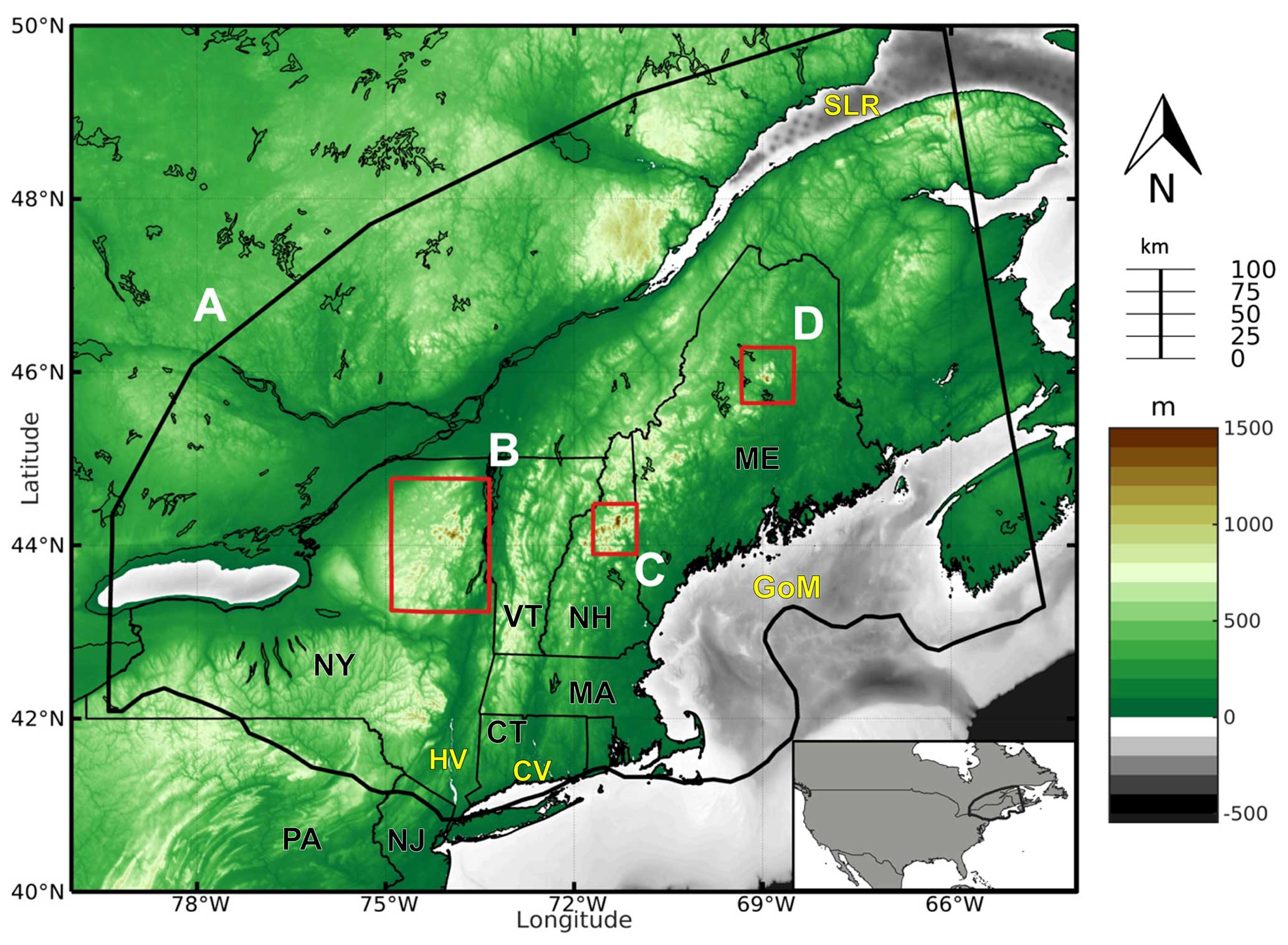
Figure 1 Bedrock topography (meters) and model domains for the regional NE USA ice sheet model (shown with black outline; a) and the local-scale models shown with the red outlines across the Adirondack Mountains (b), White Mountains (c), and Mount Katahdin (d). The southern boundary of the NE USA model (a) follows the reconstructed LGM ice extent during the LGM from Dalton et al. (2020). States are abbreviated as follows: PA – Pennsylvania, NJ – New Jersey, CT – Connecticut, NY – New York, MA – Massachusetts, VT – Vermont, NH – New Hampshire, and ME – Maine. Other locations described in the text are abbreviated as follows: HV – Hudson Valley, CV – Connecticut Valley, GoM – Gulf of Maine, and SLR – Saint Lawrence River Valley.

Fortunately, because of the high vertical relief across the NE USA, studies have addressed the vertical-thinning history of the LIS in this region by dating glacial features along vertical transects (herein referred to as dipstick studies; Bierman et al., 2015; Koester et al., 2017, 2021; Barth et al., 2019; Corbett et al., 2019; Halsted et al., 2023). Geologic archives such as glacial erratics, striations, and soil development, as well as isotopic evidence from terrestrial cosmogenic nuclide (TCN) surface exposure ages, can be interpreted to reflect subglacial thermal regimes (i.e., cold- or warm-based ice) in the past. Glacial erratics found on the peaks indicate continental ice cover at some point during the Quaternary (De Laski, 1872; Tarr, 1900; Antevs, 1932; Davis, 1989). TCN surface exposure ages from erratics and glacially affected bedrock on the peaks indicate that rapid vertical ice sheet thinning occurred coincidentally with ice margin retreat during the last deglaciation and, predominantly, during the Bølling–Allerød warm period. Through surface exposure dating of bedrock features and glacial erratics, these dipstick studies commonly find the presence of inherited nuclides across high-elevation sites (> 1200 m; Halsted et al., 2023), making geologic interpretations of the onset of vertical ice thinning at these locations uncertain. Consequently, these data suggest that the high-elevation regions of the NE USA were likely to be covered by cold-based ice characterized by the absence of subglacial water and, ultimately, much reduced subglacial erosion, with warm-based ice and erosive conditions flanking the valleys of these high-elevation regions (Halsted et al., 2022). Glacial striations and roches moutonnées found below the summits of the Presidential Range in New Hampshire (NH) and Mt. Katahdin in Maine (ME) indicate the presence of warm-based ice locally (Goldthwait, 1970; Davis, 1978, 1989; Thompson et al., 1999). Similar evidence, with the addition of weakly developed soils on the summits of the Presidential Range, indicates cover by erosive, warm-based ice (Goldthwait, 1970).

While these geologic interpretations support the existence of polythermal ice conditions across the NE USA, it is not well known how this subglacial regime varied spatially and whether the existence of this boundary occurred along a geographically consistent elevation. Furthermore, a lack of precise age control for many of these features leaves the questions of temporal variability and of whether or not the thermal regime was consistent throughout glaciation and deglaciation unanswered. This has implications for interpreting the geologic data of past ice sheet retreat or thinning, particularly at high elevations, as well as of erosional processes that may have operated during glaciation across the NE USA as erosional patterns are closely related to the ice sheet thermal regime (Lai and Anders et al., 2021). Ultimately, where these geologic archives are limited in their spatial coverage, ice sheet models can be used to simulate broader characteristics of this thermal regime.

Ice sheet models have been important tools to study LIS conditions during the Last Glacial Maximum (LGM) and to assess the drivers of deglacial change (Sugden, 1977; Marshall et al., 2000; Hooke and Fastook, 2007; Tarasov and Peltier, 2007; Gregoire et al., 2012; Moreno-Parada et al., 2023). Ice sheet models do not only aid in the interpretation of geologic proxies of past ice sheet behavior but also provide outputs that enable a more informed choice when considering field locations for sampling. For example, a recent assessment of the basal thermal state of the Greenland Ice Sheet (MacGregor et al., 2016, 2022), which, in part, relied upon outputs from newer-generation ice sheet models, was used to inform field campaigns aimed at sampling subglacial bedrock in portions of the Greenland Ice Sheet that were estimated to be cold-based with low erosion (Briner et al., 2022).

With regards to the LIS, prior ice sheet modeling efforts were useful in identifying a broad picture of the thermal behavior of the LIS, which indicated that, during the LGM, roughly 20 %–50 % of the LIS was warm-based (Marshall and Clark, 2002; Tarasov and Peltier, 2007), including the NE USA. Some aspects of these simulations (Tarasov and Peltier, 2007) do agree well with broad-scale geomorphic indicators of basal conditions (Klemen and Hattestrand, 1999; Briner et al., 2006; Klemen and Glasser, 2007; Briner et al., 2014), which indicate that the LIS exhibited a varying subglacial thermal regime, with frozen-bed patches being particularly interspersed along ice divides and, in some cases, residing along sharp boundaries with warm-based ice streams or outlet glaciers.

However, due to the low spatial resolution of existing models (> 20 km), the high topographic relief across the NE USA is poorly resolved, and, therefore, the sharp thermal boundary between cold- and warm-based ice identified in the geologic archives is not captured. This is likely due to the more coarsely resolved models' inability to capture advective and diffusive processes at these small spatial scales. Likewise, as the high relief of this region served as a control and impediment to ice flow during the LGM, the impacts of ice flow on deformational and frictional heating are more poorly captured in lower-resolution models. This can be improved by downscaling ice sheet models to a higher resolution, which has shown promise (Staiger et al., 2005) in interpreting how polythermal ice conditions may have influenced regional glacial geomorphology.

To address this shortcoming, we use a high-resolution ice sheet model to simulate the thermal regime of the LIS across the NE USA during the LGM. Our model experiments are designed to test whether the presence of this sharp thermal regime is simulated and to assess the spatial and elevational characteristics of the basal thermal regime at regional and local scales (i.e., mountain ranges) where geologic archives suggest the existence of polythermal conditions. Through this work, we aim to evaluate current geologic interpretations while also filling gaps in our understanding of this complex thermal regime, where geologic constraints are limited.

2 Methods

2.1 Modeling approach and setup

The NE USA (Fig. 1) is marked by a high topographic relief that spans an elevational range from sea level to > 1500 m. In order to capture these large gradients in the bedrock topography and thermal boundaries within the ice sheet, we employ a nested modeling approach (Briner et al., 2020; Cuzzone et al., 2022), whereby a more coarsely resolved and larger model provides the boundary conditions necessary for downscaling over regional- and local-scale domains that are more finely resolved (see Fig. S1 in the Supplement).

2.1.1 Ice sheet model

We use the Ice-sheet and Sea-level System Model (ISSM; Larour et al., 2012), a higher-order thermomechanical finite-element ice sheet model, to simulate the LIS LGM conditions across the NE USA. Because of the high topographic relief across this region and the associated impact on ice flow, we use a higher-order approximation to solve the momentum balance equations (Dias dos Santos et al., 2022). This ice flow approximation is a depth-integrated formulation of the higher-order approximation of Blatter (1995) and Pattyn (2003), which allows for an improved representation of ice flow compared with more traditional approaches in paleo ice flow modeling (e.g., shallow-ice approximation or hybrid approaches).

An enthalpy formulation that simulates both temperate and cold-based ice (Aschwanden et al., 2012; Serrousi et al., 2013; Rückamp et al., 2020) is used to capture the thermal state of the ice sheet. Our model contains four vertical layers and uses quadratic finite elements (P1 × P2) along the z axis for the vertical interpolation following Cuzzone et al. (2018) in order to better capture sharp thermal gradients near the base and to simulate the vertical distribution of temperature within the ice. This methodology has been successfully applied to simulate the transient behavior of the Greenland Ice Sheet across geologic timescales and the contemporary period (Briner et al., 2020; Smith-Johnsen et al., 2020; Cuzzone et al., 2022). The ice rheology follows Glen's flow law, with the ice viscosity being dependent on the simulated ice temperature following rate factors in Cuffey and Paterson (2010). Surface temperature (see Sect. 2.1.3) and geothermal heat flux (Shapiro and Ritzwoller, 2004) are imposed as boundary conditions in the thermal model. We use a linear friction law (Budd et al., 1979), where the basal drag (τ_b) is represented as follows:

$$\begin{array}{}\text{(1)}& {\mathit{\tau }}_{\mathrm{b}}=-{\mathit{\alpha }}^{\mathrm{2}}N{u}_{\mathrm{b}},\end{array}$$

where α represents the spatially varying friction coefficient, N represents the effective pressure, and u_b is the basal velocity. Here, $N=g({\mathit{\rho }}_{i}H+{\mathit{\rho }}_{\mathrm{w}}{Z}_{\mathrm{b}}$), where g is gravity, H is ice thickness, ρ_i is the density of ice, ρ_w is the density of water, and z_b is bedrock elevation following Cuffey and Paterson (2010). N evolves as the ice sheet thickness changes. The spatially varying friction coefficient (α) is constructed as a function of bedrock elevation above sea level (Åkesson et al. 2018; Cuzzone et al., 2024b):

$$\begin{array}{}\text{(2)}& \mathit{\alpha }=\mathrm{200}\times {\displaystyle \frac{min[max(\mathrm{0},z_{\mathrm{b}}+\mathrm{600}),z_{\mathrm{b}}]}{max\left(z_{\mathrm{b}}\right)}},\end{array}$$

where z_b is the height of the bedrock with respect to sea level. Using this parameterization, basal friction is larger across high topographic reliefs and lower across valleys and areas below sea level, which is consistent with what is found today for the Greenland Ice Sheet. The thermomechanical coupling captures the impact of ice deformation and frictional heating on ice temperature, which, in turn, affects the ice rheology through the temperature-dependent rate factor. In our approach, the friction coefficient is independent of the thermal state, but this has been explored recently in modeling LIS LGM conditions (Moreno-Parada et al., 2023). Although it is found to have a measurable impact on the overall simulated LGM ice volume, basal temperatures, and ice stream extent, particularly for Hudson Bay, these variations are small when compared with uncoupled simulations, particularly across the NE USA.

The motion of the ice front is tracked using the level set method described in Bondzio et al. (2016), and calving is simulated where the LIS interacts with the ocean based on the Von Mises stress criterion (Morlighem et al., 2016). This approach approximates the calving rate as a function of the tensile stresses simulated with the ice, with ice front retreat occurring when the Von Mises tensile strength exceeds user-defined stress thresholds set for tidewater (1 MPa) and floating ice (200 kPa). These values are consistent with other contemporary and paleo ice sheet modeling studies (Bondzio et al., 2016; Morlighem et al., 2016; Choi et al., 2021; Cuzzone et al., 2024b).

Glacial isostatic adjustment (GIA) is not simulated transiently but is instead prescribed by using a reconstruction of relative sea level from a global GIA model of the last glacial cycle (Caron et al., 2018). Bedrock vertical motion, eustatic sea level, and geoid change during the LGM are applied to our model to account for GIA (Briner et al., 2020; Cuzzone et al., 2024b).

2.1.2 Model domains

To constrain the model boundary conditions necessary for simulating the LIS conditions across the NE USA at both a regional (Fig. 1, domain A) and local scale across the Adirondack Mountains, White Mountains, and Mount Katahdin (Fig. 1, domains B–D), we first simulate the LGM ice conditions across the LIS (Fig. S1). Our model domain follows the LGM ice extent reconstructed from Dalton et al. (2020) but does not include the Cordilleran Ice Sheet and the connection between Ellesmere Island and the Greenland Ice Sheet. The LIS model is built on a structured mesh with a spatial resolution of 20 km. Bedrock topography is initialized from the General Bathymetric Chart of the Oceans (GEBCO; GEBCO Bathymetric Compilation Group, 2021), which relies on the 15 arcsec (450 m resolution) Shuttle Radar Topography Mission data (SRTM15_plus; Tozer et al., 2019) for the terrain model. The regional ice sheet model domain (Fig. 1, domain A; Fig. S1, domain 2) covers the NE USA and extends into portions of southern and maritime Quebec. Across this domain, anisotropic mesh adaption is used to construct a non-uniform mesh that varies based upon gradients in bedrock topography from GEBCO. The spatial resolution varies from 5 km in areas of low topographic relief, where gradients in bedrock topography are low, to 500 m in areas of high topographic relief. To gain a more detailed reconstruction of the LGM conditions across the NE USA that is more consistent with the spatial scales associated with the geologic archives (Halsted et al., 2023), we dynamically downscale our results to three local areas within the NE USA (Sect. 2.2; step 3): the Adirondack Mountains, New York; the White Mountains, New Hampshire; and Mount Katahdin, Maine. The local-scale models (Fig. 1, domains B–D; Fig. S1, domain 3) also rely on anisotropic mesh adaptation, with a spatial resolution varying from 400 to 30 m based upon topography from the 1 arcsec (∼ 30 m resolution) SRTM product (Farr et al., 2007). The three locations were chosen based on their geomorphic qualities as each represents three of the highest peaks in the NE USA and has pre-existing geochemical data on glaciation (e.g., cosmogenic surface exposure ages; Bierman et al., 2015; Barth et al., 2019). At these spatial scales, the model is able to resolve the high topographic relief found between the mountain peaks and neighboring valley floors.

2.1.3 Climate forcing and surface mass balance scheme

The outputs of monthly mean LGM temperature and precipitation from five different climate models are used as surface boundary conditions and to estimate the surface mass balance (SMB). The LGM climate from the TraCE-21ka transient simulation of the last deglaciation is used (Liu et al., 2009; He et al., 2013), along with the outputs from four models participating in the Paleoclimate Modelling Intercomparison Project 4 (PMIP4; Kageyama et al., 2021). The simulated climate from these models differs with respect to both the magnitude and the spatial distribution of glacial temperature and precipitation change relative to the preindustrial climate (Fig. S2 in the Supplement). By using a diverse range of surface climate forcings rather than the multi-model mean, we aim to construct a small ensemble of results for the simulated LGM conditions across our model domains as the representative climate model spread can impact the simulated ice sheet geometry, ice flow, and thermal characteristics (Lai and Anders, 2021).

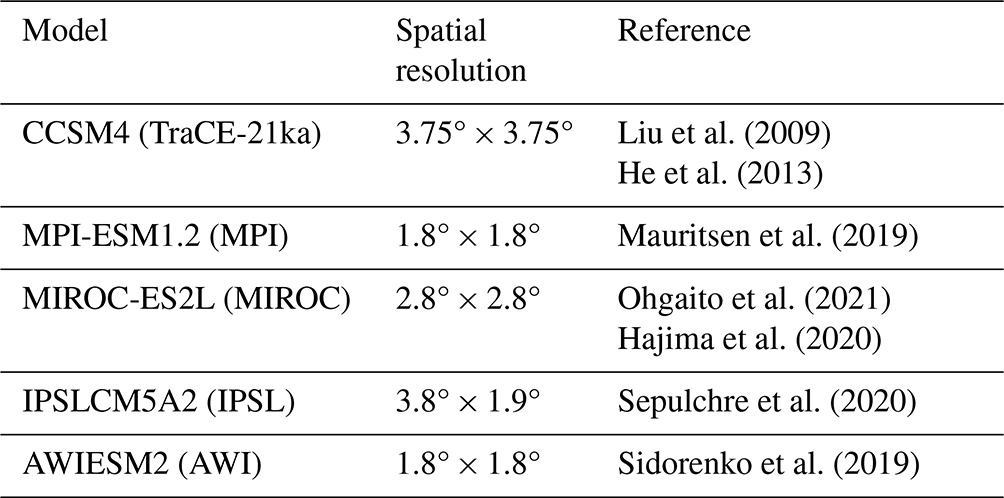
We use a positive degree day model (Tarasov and Peltier, 1999; Le Morzadec et al., 2015; Cuzzone et al., 2019; Briner et al., 2020) to calculate the SMB. Our degree day factor for snow melt is 5 and 9 $\mathrm{mm}\mathrm{°}{\mathrm{C}}^{-\mathrm{1}}{\mathrm{d}}^{-\mathrm{1}}$ for bare ice melt, and we use a lapse rate of 5 °C km⁻¹ to adjust the temperature of the climate forcings to surface elevation (Abe-Ouchi et al., 2015). The hourly temperatures are assumed to have a normal distribution, with a standard deviation of 3.5 °C around the monthly mean. An elevation-dependent desertification is included (Budd and Smith, 1981), which reduces precipitation by a factor of 2 for every kilometer change in ice sheet surface elevation, and the model accounts for the formation of superimposed ice following Janssens and Huybrechts (2000). The degree day model requires inputs of monthly temperature and precipitation. We apply a commonly used modeling approach to scale a contemporary climatology of temperature and precipitation back to the LGM (anomaly method; Pollard and DeConto, 2012; Seguinot et al., 2016; Golledge et al., 2017; Tigchelaar et al., 2019; Briner et al., 2020; Cuzzone et al., 2022). The monthly mean climatology of temperature and precipitation for the period 1979–2010 from the European Center for Medium-Range Weather Forecasts ERA5 reanalysis (Hersbach et al., 2020) is bilinearly interpolated onto our model mesh. Next, anomalies of the monthly mean temperature and precipitation fields from the climate models (Table 1), computed as the difference between the LGM and preindustrial control run, are added to the contemporary monthly mean climatology to produce the monthly temperature and precipitation fields during the LGM.

Table 1 List of climate models used for the LGM surface climate forcing and the corresponding spatial resolution.

2.2 Experimental setup

Our downscaling approach is conducted in three steps and is summarized as a flowchart in Fig. S3 in the Supplement:

Step 1 (LIS models; Figs. S1 and S4 in the Supplement)

First, we construct a model of the LGM LIS using a 2D model, with a setup as described above, and prescribe a constant LGM climate (Sect. 2.1.3). Following Moreno-Parada et al. (2023), we initialize our model with an ice thickness of 1000 m north of 50° N and allow the simulated LIS to reach equilibrium with respect to ice volume (∼ 50 000 years). The resulting models (ice geometry and velocity) are used to initialize a 3D model that extrudes the 2D model to four vertical layers (P1 × P2 vertical finite elements; Sect. 2.1.1). The thermal regime is assumed to be in a steady state in relation to the LGM climate, and we perform a thermomechanical steady-state calculation with a fixed ice sheet geometry and impose surface temperature as Dirichlet boundary conditions until the ice sheet velocities are consistent with ice temperature (i.e., convergence) following Seroussi et al. (2013). Lastly, we let the 3D LIS model relax an additional 20 000 years (i.e., until thermal equilibrium is reached) with the LGM climate as the model adjusts to the updated ice temperature and rheology.

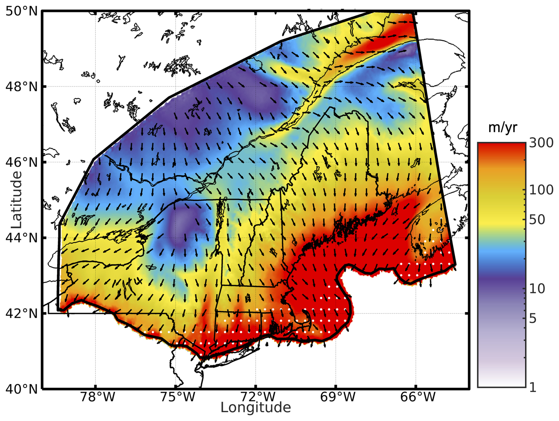
Figure 2 The modeled mean (n=5; Table 1), simulated LGM depth-integrated ice velocity (m yr⁻¹), and simulated LGM ice thickness (m) across the NE USA. Vectors illustrate the simulated direction of ice flow, and colors denote the magnitude of ice velocity. White stippling indicates areas where some individual models (see Fig. S5) simulate no LGM ice cover.

Step 2 (NE USA models; Fig. 1)

We construct our 3D NE USA ice models following the setup discussed in Sect. 2.1 and initialize the model with ice geometry, temperature, rheology, and velocity from the resulting LGM 3D LIS model. Boundary conditions of temperature, ice velocity, and thickness from the LIS results are imposed as Dirichlet boundary conditions at the western, northern, and eastern boundaries following Cuzzone et al. (2022). The initial ice velocity and temperature are downscaled across this domain by performing a thermomechanical steady-state calculation (Seroussi et al., 2013). The model is then allowed to relax with a constant LGM climate for 20 000 years as the ice geometry, flow, and temperature adjust to the higher-resolution grid.

2.2.1 Step 3 (local models; Fig. 1)

Similarly to step 2, the local-scale models are initialized with ice geometry, temperature, rheology, and flow, with the results from the NE USA model (as in step 2) and the boundary conditions from the NE USA model (as in step 2) being applied to the local-scale models at the northern, southern, eastern, and western boundaries. After running a thermomechanical steady-state calculation, the model is allowed to relax to a steady state with a constant LGM climate as the ice geometry, flow, and temperature adjust to the higher-resolution grid.

The approach outlined above makes use of the thermomechanical steady-state calculation to avoid high computational expense in relaxing the 3D models for a sufficiently long time (e.g., > 100 000 yr) until thermal equilibrium is reached. This methodology has been applied to study the basal temperature of present-day ice sheets (Seroussi et al., 2013; MacGregor et al., 2016, 2022), and, although it assumes that the ice sheet is in equilibrium with climate, we acknowledge that the thermal conditions of the LIS during the LGM likely reflect the transiently evolving ice geometry and climatic conditions experienced during the growth and advance to the LGM maximum. For this study, we focus the discussion of our results on the simulated LGM state of the NE USA models (step 2) and local models (step 3), but we refer the reader to Fig. S4 for an illustration of the simulated LGM state of the LIS (step 1).

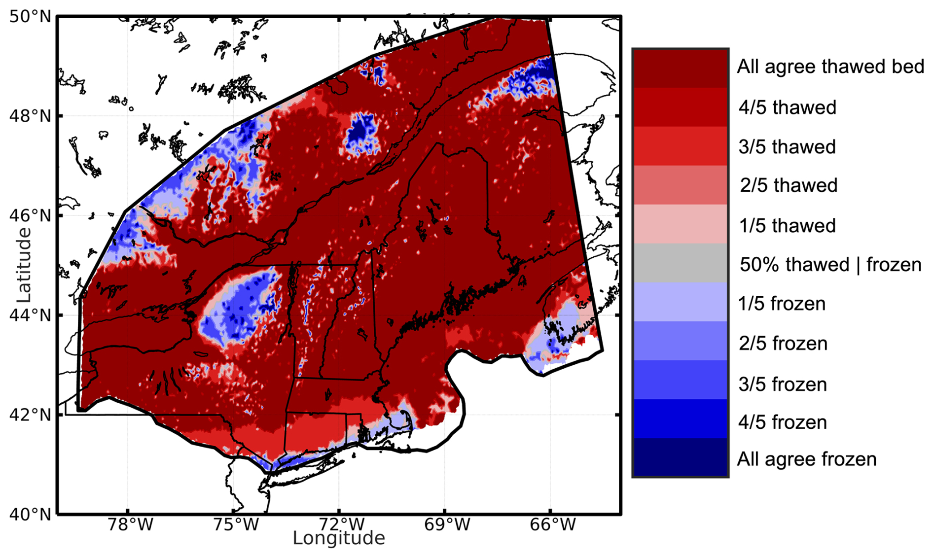
Figure 3 The agreement in the simulated LGM basal thermal state (n=5) for the experiments with varying climate forcing. We assume that a thawed bed is present when the pressure-corrected T_bed ≥ −1 °C and that the frozen bed is present when T_bed < −1 °C, following MacGregor et al. (2022).

3 Results

3.1 Northeastern USA

We simulate a range of possible LGM states given different climatologies and do not specifically tune our models to match reconstructions of ice extent or flowlines. The southern boundary of our model domain is constrained to the maximum reconstructed LGM ice extent from Dalton et al. (2020). In total, we have five different simulations of the LIS across the NE USA during the LGM (Fig. S5 in the Supplement), driven by the independent climate forcings (Table 1). The depth-integrated ice velocity and ice thickness for the ensemble mean (n=5) of those experiments are shown in Fig. 2. Individually, most of the experiments simulate an LGM ice margin that reaches the reconstructed terminal LGM ice extent (Figs. 2b and S5) from Dalton et al. (2020), although some simulate reduced ice extent, particularly along the southern and eastern boundaries (Fig. S5). Thinner ice (< 500 m) is found along the ice margin and along marine-terminating portions of the Atlantic Ocean and the Gulf of Maine, and this thickens to more than 3500 m over the northwestern portion of the model domain. Across the northwestern region, ice velocities are slow (< 20 m yr⁻¹), consistently with a northward-trending ice divide simulated through Quebec (see Fig. S4). Additionally, a regional ice divide is simulated across the Adirondack Mountains (Fig. 2), where ice velocities are < 15m yr⁻¹ and where ice flow vectors indicate diverging ice flow to the southwest and southeast. This regional ice divide is simulated for all experiments (Fig. S5), with variation in the magnitude of the ice velocities (∼ 1–25 m yr⁻¹). Faster ice flow (> 50 m yr⁻¹) is found along the ice margin and through areas of topographic troughs. Horizontal ice flow is fastest in marine-terminating portions, such as in the Gulf of Maine (GoM; Fig. 1), in the St. Lawrence River (SLR; Fig. 1), and throughout lower terrain such as the Hudson and Connecticut river valleys (HC, CV; Figs. 1 and 2), with speeds approaching and exceeding 300 m yr⁻¹.

For each experiment, we calculate the simulated basal temperature, adjusted for pressure melting (i.e., pressure-corrected temperature). Following MacGregor et al. (2022), we consider a thawed bed to be simulated where the pressure-corrected T_bed ≥ −1 °C, and we consider the bed to be frozen where T_bed < −1 °C. The magnitude of the simulated thawed- and frozen-bed conditions varies across our model domain (Fig. S5) but follows a spatial pattern that can be summarized in Fig. 3, where we show the inter-model agreement between experiments for thawed- and frozen-bed conditions. We find that approximately 70 % of the model domain is thawed and that only 2 % of the model domain has frozen-bed conditions (i.e., area of the domain where all experiments agree), indicating that warm-based ice conditions prevailed across this portion of the LIS.

Warm-based areas are coincident with areas of fast ice flow (Fig. 2), where sliding dominates. Frozen-bed conditions are generally simulated in areas of reduced ice flow (< 15 m yr⁻¹; Fig. 2), particularly along the ice divide that exists in the northwestern portion of the model domain, south of the St. Lawrence River, and across the Adirondack Mountains. Additionally, the regional model simulates the presence of cold-based ice scattered across areas of high bedrock elevation (see Fig. 1 for topographic map). In general, each experiment using the different climate surface forcings simulates a similar spatial pattern of warm-based and cold-based ice (Fig. S5). Each experiment disagrees with respect to the magnitude of basal cooling, with some experiments simulating both colder basal temperatures and a wider swath of frozen-bed conditions, primarily across the Adirondack Mountains (Fig. S5; TraCE-21ka, MPI, and IPSL). This is likely to be related to the differences in the simulated LGM surface climate between each climate model. The experiments which simulate a larger swath of frozen-bed conditions across the Adirondack Mountains (Fig. S5; TraCE-21ka, MPI, and IPSL) have a higher magnitude of simulated LGM surface cooling and a higher SMB (Fig. S6 in the Supplement; TraCE-21ka, MPI, and IPSL) versus the experiments which simulate less extensive frozen-bed conditions across the Adirondack Mountains (Figs. S5 and S6; MIROC and AWI).

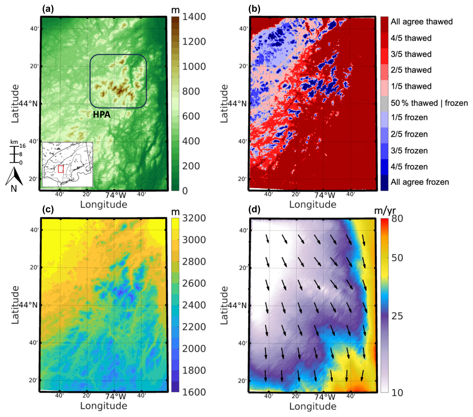
Figure 4 (a) Bedrock topography of the Adirondack Mountains (m). Box highlights the high-peak area. See inset in Fig. 4a for geographical context within the NE USA. (b) Modeled agreement for simulated frozen- and thawed-bed conditions. (c) The model mean ice thickness (m). (d) The model mean depth-averaged ice velocity (m yr⁻¹). Note, vectors denote ice flow direction and not the magnitude of velocity.

3.2 Local models

3.2.1 Adirondack Mountains

The simulated mean (n=5) LGM conditions for the Adirondack Mountains are presented in Fig. 4. A high topographic relief that exceeds 1000 m is characteristic of the Adirondack Mountains, with 43 mountain peaks exceeding 1200 m in elevation and maximum elevations reaching 1600 m (Fig. 4; HPA: high-peak area). The simulated LGM ice thickness reaches between 1600 to 2000 m across the highest peaks, increases throughout the lower valleys to be in excess of 2000 m, and reaches upwards of 3000 m across the lower elevations in the northwestern and northeastern portions of the domain (Fig. 4c). Consistently with the ice divide simulated in the regional model (Fig. 2), slow ice velocities (< 10 to 25 m yr⁻¹) dominate across the Adirondack Mountains (Fig. 4d). Ice flow generally trends in a south–southeastward direction, with ice velocities increasing to > 60 m yr⁻¹ across lower-elevation valleys. Approximately 58 % of the model domain is thawed, and 4 % of the model domain has frozen-bed conditions (i.e., area of domain where all experiments agree), indicating that warm-based ice conditions prevailed across this portion of the LIS (Fig. 4e). Generally, frozen-bed conditions are confined to high-elevation peaks (Fig. 4b), where low ice velocities and thinner ice exist, making these high-elevation regions more susceptible to vertical advection of cold surface temperatures (LGM temperatures range between climate models: −24 to −18 °C). However, we also find that, across lower-elevation regions, particularly in the northwestern portion of the domain, frozen-bed conditions are simulated. Here, ice is thick (upwards of 3000 m; Fig. 4a) but is characterized by very slow ice flow (< 10 m yr⁻¹). Without limited frictional and deformational heating, this area was likely to be influenced by the vertical advection of cold surface climate despite thick ice. Across this domain, the thermal boundary separating frozen and thawed beds (Fig. 4e) is 880 m. However, if we consider only the high-peak area (HPA; Fig. 4a), that thermal boundary resides at 1180 m.

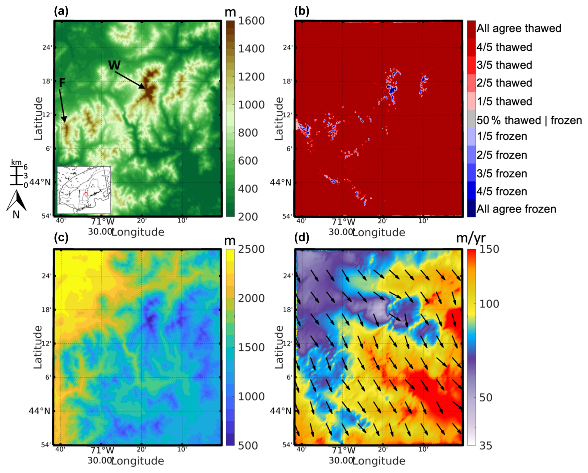
Figure 5 (a) Bedrock topography for the White Mountains (m). Highlighted are Mt. Washington (W) and Mt. Lafayette and Little Haystack Mountain, labeled (F) for Franconia Range. See inset in Fig. 5a for geographical context within the NE USA. (b) Modeled agreement for simulated frozen- and thawed-bed conditions. (c) The model mean ice thickness (m). (d) The model mean depth-averaged ice velocity (m yr⁻¹). Note that vectors denote ice flow direction and not the magnitude of velocity.

3.3 White Mountains

To the east of the Adirondack Mountains, the White Mountains comprise a series of mountain ranges intersected by deeply incised valleys, with the highest peak, Mount Washington, reaching 1912 m (Fig. 5a). The simulated mean LGM conditions for the White Mountains are presented in Fig. 5. Ice thickness ranges between 600 to 1200 m across high-elevations peaks (Fig. 5c), and it reaches 2000 m in the deeply incised valleys. Across the lower elevations in the northwestern portion of the model domain (Fig. 5a), ice thickness reaches upwards of 2500 m. Ice flows southeastward across this region, with simulated ice velocities being higher than what is found across the Adirondack Mountains. Ice velocities are lowest in the northwestern portion of the domain and across Mount Washington, where the southeastward ice flow is impeded by the high-elevation bedrock (35–60 m yr⁻¹; Fig. 5d) and increases to up to 150 m yr⁻¹ across the lower elevations in the southeastern region. When considering the basal thermal regime, we find that 95 % of the model domain has thawed-bed conditions, with only 0.5 % of the domain having frozen-bed conditions. Frozen-bed conditions are limited to high-elevation sites, particularly across the Presidential Range, where Mount Washington is located, and across Mount Lafayette and Little Haystack in the Franconia Range, with a mean thermal boundary between frozen- and thawed-bed conditions residing at 1530 m.

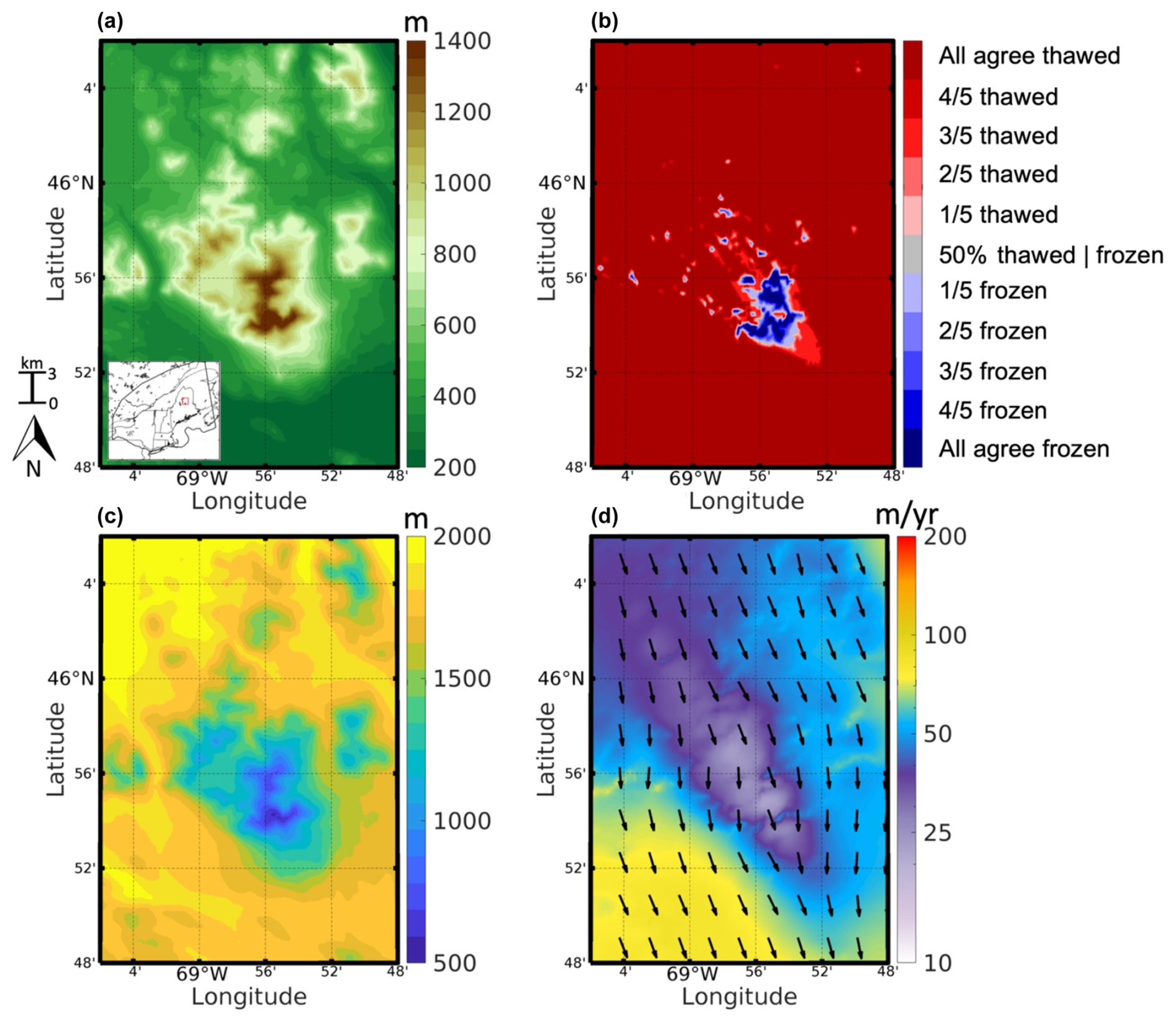
Figure 6 (a) Bedrock topography for Mount Katahdin (m). See inset in Fig. 6a for geographical context within the NE USA. (b) Modeled agreement for simulated frozen- and thawed-bed conditions. (c) The model mean ice thickness (m). (d) The model mean depth-averaged ice velocity (m yr⁻¹). Note that vectors denote ice flow direction and not the magnitude of velocity.

3.3.1 Mount Katahdin

Mount Katahdin reaches 1606 m, with more than 1300 m in relief above the surrounding valleys (Fig. 6a). The simulated mean LGM conditions for Mount Katahdin are presented in Fig. 6. Across the summit of Mount Katahdin, ice thicknesses reach between 500–700 m and thicken to 1500–2000 m around the flanks of the mountain (Fig. 6c) and the surrounding lowlands. The ice generally flows south–southeastward (Fig. 6d), with ice flow diverging and slowing down to 25 m yr⁻¹ upstream of Mountain Katahdin before reaching a minimum of 10–15 m yr⁻¹ at the summit. Ice flow converges on the downstream side of Mount Katahdin and reaches 50–100 m yr⁻¹ across the lower elevations to the south and east. The simulated basal thermal regime indicates that approximately 97 % of the domain is thawed (Fig. 6e), with only a few locations across the summit of Mount Katahdin having frozen-bed conditions, representing ∼ 0.5 % of the model domain. The elevational boundary separating frozen- and thawed-bed conditions across this domain is simulated to be at 1320 m.

4 Discussion

Across the broader LIS, geomorphic and cosmogenic isotopic evidence supports the existence of frozen-bed conditions interspersed amongst regions of warm-based ice (Klemen and Hattestrand, 1999; Klemen and Glasser, 2007; Marquette et al., 2004) and along southern sectors of the LIS, where ice cover was thin (Colgan et al., 2002). More regional indicators of polythermal conditions, with sharp contacts of warm-based ice in fast-flowing outlet glaciers and of cold-based ice on the slow-moving ice of the uplands, have been found across Arctic Canada and Baffin Island (Davis et al., 1999, 2006; Marsella et al., 2000; Briner et al., 2006, 2014; Corbett et al., 2016). Prior to direct evidence from surface exposure dating (Bierman et al., 2015), it was unknown whether cold-based ice may have existed across the NE USA. Ice sheet models have been used to infer the basal thermal conditions of the LIS, with implications for better understanding large-scale and regional ice flow and controls on ice mass evolution and regional geomorphology (Sugden et al., 1977; Marshall and Clark, 2002; Tarasov and Peltier, 2007; Moreno-Parada et al., 2023). However, while these models provide possible scenarios for the LGM and the deglacial evolution of the LIS thermal state, the coarse spatial resolution of existing models limits the ability to capture sharp thermal gradients that may have existed in high-relief terrain, with models simulating large-scale warm-based conditions during the LGM across the NE USA (Tarasov and Peltier, 2007). Our downscaled, local simulations agree with geologic interpretations (Davis, 1989; Bierman et al., 2015; Corbett et al., 2018; Halsted et al., 2023) that suggest that cold-based ice existed across areas of high relief in the NE USA and that polythermal ice existed in the region during the LGM. While the majority of this region was exposed to warm-based ice conditions (70 %; Fig. 3), frozen-bed conditions are simulated across areas of low ice velocity (i.e., ice divides) and high elevations (2 % of area in Fig. 3). It is worth noting that, while the focus of this study was on the NE USA, areas of frozen-bed ice conditions are simulated for portions of maritime Canada (Fig. 3), agreeing reasonably well with geologic interpretations from this region (Olejczyk and Gray, 2007).

Because a majority of the geologic data constraining the thermal regime of the LIS across this region are found in areas of high relief, we focused our modeling on three specific locations. Regionally, geologic interpretations posit that the Adirondack Mountains may have acted as an impediment to the south–southeastern flow of the LIS during glacial expansion and the LGM (Franzi et al., 2016). Our simulations suggest that ice flow across this region was slow (< 15 m yr⁻¹; Figs. 2a and 4a) in response to a divergence of ice flow around the mountainous terrain. Consequently, a regional ice divide and frozen-bed conditions are simulated across portions of this region, where ice velocities are < 10 m yr⁻¹, and in areas where the bedrock relief is high. This is further supported by the individual model experiments. Those experiments with colder LGM boundary conditions and higher accumulation simulated higher SMB (Fig. S6; TraCE-21ka, MPI, and IPSL) and, therefore, resulted in a stronger magnitude and a wider swath of cold-based ice conditions across the Adirondack Mountains (Fig. S5; TraCE-21ka, MPI, and IPSL). Such conditions are similar to what has been reported to exist across the thick ice divides of modern ice sheets (i.e., Greenland Ice Sheet; MacGregor et al., 2022), where, in the absence of heat generation due to frictional heating, vertical advection of cold surface climate dictates the basal thermal state (Lai and Anders, 2021). We also find that frozen-bed conditions existed across other areas of high bedrock relief during the LGM (Fig. 3), where frozen-bed patches are simulated above warm-based ice at lower elevations. Across both the White Mountains and Mount Katahdin (Figs. 5 and 6), upstream ice flow slowed as it encountered resistance from the underlying high bedrock relief. Only where both ice velocity and thickness are relatively low and where bedrock elevation is high is the presence of frozen-bed conditions simulated. Where ice thickness and driving stresses increase downstream of these bedrock features, ice velocities increase, and warm-based conditions are simulated. We note that, while the impact of degree day factors is unexplored in this work, we expect this to have a limited influence on the simulated thermal characteristics of the LIS across the NE USA. During the LGM, monthly surface temperatures remain below freezing across the ice sheet interior, with the exception of the southern margin (Fig. S6). Therefore, surface melt is limited across the ice sheet interior, and, instead, the prescribed surface temperature and accumulation are the primary factors driving the simulated differences in the thermal conditions (Fig. S6). Nevertheless, for simulations across the last deglaciation, the choice of degree day factors can have a large influence on the simulated ice history and, ultimately, the transient evolution of ice temperature as deglacial surface temperature and melt increase (Matero et al., 2020).

Regional geologic interpretations of isotopic data suggest that a thermal boundary between cold-based (low erosive) and warm-based (erosive) ice existed at ∼ 1200 m across areas of high bedrock relief in the NE USA (Halsted et al., 2022). Yet, undated geomorphic indicators of warm-based ice on Mount Washington are found at 1680 and 1820 m. Across Mount Katahdin and the White Mountains, we simulate a thermal boundary of 1320 and 1530 m, respectively, which is in reasonable agreement with the different geologic assessments.

Across the Adirondack Mountains, frozen-bed conditions are simulated both in areas of high bedrock relief and at lower-elevation sites that reside under a simulated regional ice divide, making the interpretation more complicated. While the region-wide thermal boundary is simulated to be at 880 m, if we only consider the high-peak area where geologic data of ice thinning exist (Barth et al., 2019), the thermal boundary resides at 1180 m. For high-elevation sites, Barth et al. (2019) present an alternative hypothesis that the high-elevation TCN ages suggest early ice sheet thinning around ∼ 20 ka in lieu of reflecting nuclide inheritance and that the regional thermal boundary likely existed above 1560 m. Nevertheless, our simulations confirm that this thermal boundary was not spatially constant and instead varied geographically (Bierman et al., 2015; Corbett et al., 2018; Koester et al., 2021).

While our experiments offer a spatially high-resolution reconstruction of the LGM basal thermal conditions of the LIS across the NE USA, our methodology assumes that the LIS is in equilibrium with the LGM surface climate, which is likely not to be a true reflection of LGM conditions. It is noted that, while Tarasov and Peltier (2007) simulate the LIS thermal state across the last glacial cycle and find that maximum areal coverage of frozen-bed conditions occurred during the LGM, since the LIS experienced a transiently evolving climate prior to the LGM as the surface climate cooled, our simulations may reflect a colder thermal state than what may have been experienced. Additionally, the spatially varying basal friction coefficient is constant and not thermodynamically coupled in our simulations. While this coupling has recently been shown to have the greatest influence in areas of ice streaming across the LIS, with attendant feedbacks on ice surface lowering and, ultimately, ice thickness, a thermodynamically coupled friction may promote colder basal conditions through feedbacks between ice flow, ice temperature, and basal friction (Moreno-Parada et al., 2023). Although we cannot fully address how these limitations and assumptions affect our results, since our simulations agree well with geologic interpretations that polythermal conditions and, ultimately, a regime of differential erosion existed across the NE USA, we attain a level of confidence that we are indeed simulating thermal conditions that generally reflected LGM conditions. However, future work should evaluate how these thermal conditions may have changed in response to deglacial LIS change as our contemporary assessment of geomorphic and geologic indicators likely integrates the full glacial and deglacial history.

Because the data derived from dipstick studies aimed at constraining vertical-thinning histories can be difficult to interpret, our regional- and local-scale modeling framework may prove to be helpful for making more informed choices with regard to sample site selection in places where model simulations suggest warm-based and, ultimately, erosive ice conditions, such as what is currently being done for fieldwork in the Adirondack Mountains (Barker et al., 2024). Additionally, since the results presented here support broader geologic interpretations that polythermal ice conditions likely existed across the NE USA (Halsted et al., 2023), such output may be useful in geomorphological interpretations of differential erosion and relief generation, as well as of transport processes of glacial erratics from lower-elevation, warm-based areas (Bierman et al., 2015). Lastly, such a framework shows promise in applications to other regions of the LIS where geologic and geomorphic indicators suggest the existence of sharp thermal contacts and erosional history, such as across portions of Arctic Canada and Baffin Island (Marsella et al., 2000; Briner et al., 2006, 2014).

5 Conclusions

In this study, we use a numerical ice sheet model to simulate, at a high spatial resolution, steady-state LGM basal thermal conditions for the LIS across the NE USA and at three specific locations characterized by high bedrock relief. LGM climate boundary conditions are used from a small ensemble of climate model simulations, each with a varying degree of LGM cooling and precipitation change relative to preindustrial climate. Our results illustrate that, during the LGM, the LIS across the NE USA was mainly warm-based and, ultimately, erosive but exhibited polythermal ice conditions as simulations reveal that cold-based ice existed across this region in areas of high bedrock elevation and slow ice flow (i.e., ice divides). At local scales, we find that, within the Adirondack Mountains, a regional ice divide is simulated during the LGM, characterized by low ice velocities (< 15 m yr⁻¹) and a wide swath of cold-based ice that spans a large elevational range. Across the White Mountains and Mount Katahdin, ice velocities are generally higher, with cold-based ice conditions being simulated only amongst the highest-elevation peaks. Where existing models (Marshall and Clark, 2002; Tarasov and Peltier, 2007; Gregoire et al., 2012) lack sufficient resolution to capture these features, we simulate a complex thermal regime that may have existed across this region, reflective of the highly variable topography.

The results presented here support the conclusions from a large dataset of TCN surface exposure ages that relate nuclide inheritance across high-relief areas of the NE USA to the presence of cold-based and low erosive conditions sometime during the LGM and last deglaciation (Bierman et al., 2015; Koester et al., 2017, 2021; Barth et al., 2019; Corbett et al., 2018; Corbett et al., 2019; Halsted et al., 2022; Halsted et al., 2023). These studies largely support the fact that a thermal boundary of ∼ 1200 m in elevation separated cold-based ice at higher elevations and warm-based ice at lower elevations. While our simulations support this conclusion, they also illustrate that this thermal boundary was not spatially consistent and instead varied geographically. The existence of polythermal ice conditions across this region has implications with respect to glacial geomorphology as the erosive character of the ice sheet is closely tied to the basal thermal regime. While dipstick studies (Bierman et al., 2015; Koester et al., 2017, 2021; Barth et al., 2019; Corbett et al., 2019; Halsted et al., 2023) have the potential to provide critical constraints on paleo ice sheet thinning, interpretations can be hindered by the existence of cold-based ice (i.e., low erosion and, thus, nuclide inheritance). Therefore, studies like this may aid in future study site selection (e.g., Briner et al., 2022; Barker et al., 2024) as this downscaling procedure can be applied to specific sites of interest. Additionally, this downscaling approach may be useful for geomorphological assessments in other areas of the LIS where polythermal conditions may have existed (Davis et al., 1999; Davis et al., 2006; Briner et al., 2014; Staiger et al., 2005) by providing another metric to evaluate landscape evolution.