Inferring the seasonality of sea ice floes in the Weddell Sea using ICESat-2

Over the last decade, the Southern Ocean has experienced episodes of severe sea ice area decline. Abrupt events of sea ice loss are challenging to predict, in part due to incomplete understanding of processes occurring at the scale of individual ice floes. Here, we use high-resolution altimetry (ICESat-2) to quantify the seasonal life cycle of floes in the perennial sea ice pack of the Weddell Sea. The evolution of the floe chord distribution (FCD) shows an increase in the proportion of smaller floes between November and February, which coincides with the asymmetric melt–freeze cycle of the pack. The freeboard ice thickness distribution (fITD) suggests mirrored seasonality between the western and southern sections of the Weddell Sea ice cover, with an increasing proportion of thicker floes between October and March in the south and the opposite in the west. Throughout the seasonal cycle, there is a positive correlation between the mean chord length of floes and their average freeboard thickness. Composited floe profiles reveal that smaller floes are more vertically round than larger floes and that the mean roundness of floes increases during the melt season. These results show that regional differences in ice concentration and type at larger scales occur in conjunction with different behaviors at the small scale. We therefore suggest that floe-derived metrics obtained from altimetry could provide useful diagnostics for floe-aware models and improve our understanding of sea ice processes across scales.

1 Introduction

Sea ice is a key resource of the climate system, shielding the ocean from solar radiation, regulating the ocean's overturning circulation (Gill, 1973), influencing lower-latitude weather (England et al., 2020; Zhu et al., 2021), shaping interactions with ice shelves (Nicholls et al., 2009), and delivering critical support functions for polar ecology (Kohlbach et al., 2018; Vernet et al., 2019; Trathan et al., 2020; Fretwell et al., 2023). While Antarctic sea ice area remained relatively stable between 1979 and 2015, the occurrence of several recent summer minima in the pack's extent (Parkinson, 2019; Turner et al., 2022; Purich and Doddridge, 2023) may be signalling a longer-term downward trend. The perennial extent of Antarctic sea ice is small compared to the seasonal portion of the pack but is particularly important for the polar ocean circulation and remains poorly understood due to sparse observations.

Over a seasonal cycle, the sea ice cover undergoes transformations that may provide insights into how the pack may respond to a changing environment. At the start of spring, solar heating initiates the melting of the pack, which facilitates the formation of leads due to stress induced by winds, ocean currents, and waves (Rampal et al., 2009). This seasonal transition toward weaker ice does not always occur linearly with the drop in ice concentration, as storms may break the pack without a notable change in basal ice area (Hutchings et al., 2012). Further fracturing generates individual pieces of ice, or floes, which respond more readily to synoptic variability in the atmosphere and fine-scale turbulence in the ocean (Horvat et al., 2016; Gupta and Thompson, 2022; Brenner et al., 2023). The characteristics of sea ice floes also evolve during the winter months due to dynamical processes including floe–floe collisions, ridging, and rafting, which redistribute sea ice mass and area across scales (Hwang et al., 2017). Currently, due to the coarse resolution of climate models, the floe-scale connections between sea ice states across a seasonal cycle remain poorly understood and contribute to biases in sub-yearly predictions of sea ice extent (Bushuk et al., 2021).

The fine-scale properties of the sea ice pack have traditionally been characterized by the floe size distribution (FSD) inferred from imagery (Rothrock and Thorndike, 1984; Toyota et al., 2006; Denton and Timmermans, 2022). FSDs evolve seasonally, reflecting the proliferation of smaller floes in spring and summer and the consolidation of the pack during winter and fall (Steer et al., 2008; Geise et al., 2017; Stern et al., 2018). A cascade of processes governs this transition (Herman et al., 2021; Hwang and Wang, 2022), including fractures due to atmosphere and ocean turbulence, wave-induced breakage, grinding due to floe–floe collisions, and lateral melt caused by peripheral oceanic heat (Steele, 1992). Sea ice floes also undergo welding, ridging, and rafting (Timco and Burden, 1997; Vella and Wettlaufer, 2007; Herman, 2012), which congeal the ice back into consolidated sheets. Theory-based inferences of sea ice fracture predict a variety of floe shapes and size distributions, but currently no single model can emulate the wide range of statistics and behaviors inferred from the observations (Herman et al., 2021; Montiel and Mokus, 2022) due to uncertainties regarding sea ice modes of failure and their applicability across scales. Recent advances in measuring fine-scale sea ice properties from altimetry and imagery have provided regional to basin-wide estimates of floe and lead statistics (Horvat et al., 2019; Farrell et al., 2020; Petty et al., 2021; Muchow et al., 2021; Koo et al., 2023). Nevertheless, the relative importance of localized vs. basin-scale forcings in governing floe-scale sea ice dynamics remains uncertain.

Challenges in interpreting sea ice behavior also stem from the paucity of ice thickness data (Giles et al., 2008; Kurtz and Markus, 2012), particularly in the Southern Hemisphere. Thicker ice is mechanically stronger (Hopkins, 1998) and can mitigate surface exchanges of heat, carbon, and light more efficiently than a thin cover (Stephens and Keeling, 2000; Gupta et al., 2020). Recent altimetric products provide high-resolution measurements of the freeboard ice thickness (Kwok et al., 2009; Laxon et al., 2013; Tilling et al., 2018; Kacimi and Kwok, 2020), which has been successfully leveraged to reduce sea ice volume biases in data-assimilated regional models (Fiedler et al., 2022; Williams et al., 2023). The ice thickness distribution (ITD) inferred from altimetry follows predictable statistical laws, but its seasonality and regional variability remain understudied (Kwok et al., 2009). Early results from representing the joint floe size and thickness distribution within climate models suggest that these fine-scale features can strongly influence the melt rate of the pack but require tighter calibration to observational inferences to produce accurate predictions (Roach et al., 2018; Boutin et al., 2020).

Our study focuses on the Weddell Sea, which hosts the most extensive perennial sea ice cover in the Southern Hemisphere (Eicken, 1992; Parkinson and Cavalieri, 2012). The physical conditions in the Weddell Sea are characterized by a large-scale gyral circulation, driven by winds, which advect sea ice in a clockwise motion across the basin to an outflow region in the northwest. This circulation favors the accumulation of sea ice along the southern rim of the basin and the eastern edge of the Antarctic Peninsula (Hutchings et al., 2012), promoting substantial amounts of multiyear sea ice in those regions. The mean thickness of this aged sea ice typically exceeds 3 m (Haas et al., 2008), rendering it some of thickest sea ice in the Southern Ocean. The wind-driven export of sea ice away from the southern Weddell Sea also regularly exposes the sea surface to cold air, allowing the formation of new ice during a large fraction of the year. The seasonal melt and freeze cycle of sea ice, combined with its gyre-driven advection, leads to complex multi-scale patterns in sea ice age, and thus properties, within the basin.

This work uses satellite-derived products to examine the seasonality of the perennial sea ice zone in the Weddell Sea and explore the utility of floe-level metrics in interpreting the larger-scale behavior of the pack. Section 2 details the datasets and methodology used in the analysis. Section 3 presents results pertaining to the seasonal evolution of sea ice types using microwave data and its floe-scale properties using the Ice, Cloud, and land Elevation Satellite (ICESat-2). Section 4 provides a discussion of the results, and Sect. 5 concludes.

2 Datasets and methods

2.1 Analysis regions

The analysis considers two distinct regions within the Weddell Sea, namely a western box (62–73° S, 45–65° W) and a southern box (73–77.6° S, 15–65° W), as shown in Fig. 2a and b. These regions were selected because they contain a significant amount of sea ice throughout the year, which allows us to consider the full seasonal cycle of sea ice floes. The western region is in contact with the Antarctic Peninsula, though a portion of it extends beyond the tip of the peninsula, toward the Antarctic Circumpolar Current (ACC). The southern region is in contact with the Filchner–Ronne Ice Shelf in the south and the Brunt and Riiser-Larsen ice shelves in the east. This region is affected by seasonal and interannual variability in sea ice properties due to polynya formation as well as dynamical blocking due to episodic grounding of very large icebergs. The area of the western region is twice as large and has a stronger north–south difference than the southern region such that they capture different sea ice regimes.

2.2 Gridded sea ice products

We use the Multiyear Ice Concentration and Ice Type (MICIT) dataset (Shokr et al., 2008; Melsheimer et al., 2023), which leverages passive brightness temperature and active microwave data to estimate daily concentrations of multiyear ice (MYI), first-year ice (FYI), young ice (YI), and open water at a nominal resolution of 12.5 km. We use the uncorrected version of the dataset, as the corrected version does not provide FYI and YI concentrations and is not available between November and March. The time series of MYI concentration in the regions of interest compare well between the two versions of the product (Fig. A1). Validation of the MICIT dataset with Sentinel-1 synthetic aperture radar (SAR) images, stage of development charts, and polynya data shows acceptable accuracy and precision, especially for Antarctic MYI at the freeze-up (Melsheimer et al., 2023). Additionally, we use the gridded sea ice freeboard obtained from the ICESat-2 ATL20 product at 25 km spatial resolution (Petty et al., 2020) and weekly gridded sea ice motion vectors at 25 km resolution from the Polar Pathfinder Version 4 dataset (Tschudi et al., 2019).

2.3 Along-track ICESat-2 altimetry

This study employs along-track data retrieved from the ICESat-2 laser altimeter (Markus et al., 2017; Neumann et al., 2019) between October 2018 and October 2022. We use sea ice freeboard measurements from the processed ATL10 version 6 product (Kwok et al., 2019, 2021) in the western and southern regions, which have a total of 3638 and 5996 tracks, respectively. We exclusively use the three sets of “strong” beams from each track, which are separated by 3 km in the across-track direction. The segment length is ∼15 m and the individual laser footprint size is ∼11 m such that the effective along-track resolution is approximately ∼26 m (Kwok et al., 2019; Petty et al., 2021). The freeboard measurements are provided relative to a local sea surface height obtained at sea ice leads within approximately 10 km of a given segment. These freeboard measurements are most reliable in areas of high sea ice concentration (>50 %; Petty et al., 2020), thus guiding our focus on the perennial ice cover.

We identify individual floes along a track according to their separation by “specular” and “dark” leads (specular leads: height_segment_type =2–5; dark leads: height_segment_type =6–9) (Kwok et al., 2022). Following past work (Horvat et al., 2019; Petty et al., 2021), we define the sea ice located between two consecutive leads along a track as a single floe and the extent of that sea ice segment as the floe chord length (Fig. 1). The mean freeboard of each sea ice floe is also calculated.

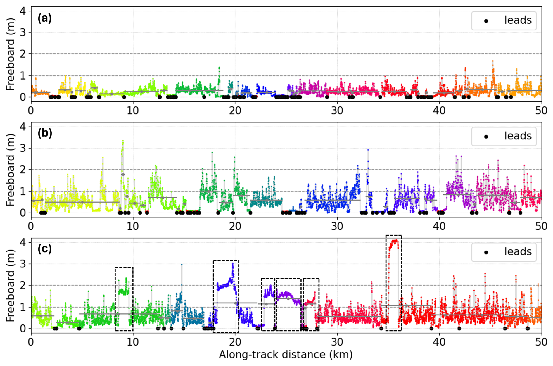
Figure 1 Identification of sea ice floes from along-track freeboard profiles of the ATL10 products taken on (a) 9 March 2019, (b) 16 September 2019, and (c) 23 October 2019. Black dots indicate the location of specular and dark leads detected by the ATL07/10 products. Different colors indicate individual floes identified based on two consecutive leads (black dots). The horizontal gray lines show the length of individual floes and the gray dots indicate their mean freeboard value. In the track shown in panel (c), the segments displaying relatively smooth and high freeboard values likely indicate the presence of broken-up landfast ice (dashed boxes).

We note that several thick ice bodies, such as broken landfast ice or small icebergs, may remain in some ICESat-2 track data despite the iceberg filtering included in the ATL07/10 products (Kwok et al., 2022, 2023). These pieces of broken landfast ice and small icebergs typically have smoother and larger freeboard values, which can be visually distinguished from sea ice floes. Here, we do not seek to precisely identify all these thick ice bodies in our tracks but rather estimate their approximate number to ascertain how they may affect our results. We first collect all the tracks comprising more than five floes whose mean freeboard height is greater than 1 m. We then manually count thick ice bodies within these tracks by visually identifying segments that have uncharacteristically smooth and high freeboard profiles (Fig. 1c). In the year 2019, we find that only 0.12 % of the detected sea ice floes (397 out of 314 582) are affected by the presence of thick ice bodies such that these likely do not significantly impact the results presented in Sect. 3.

Given the horizontal resolution of ICESat-2, the minimum floe size considered in this work is 25 m. We also note that the ATL07/10 lead detection product does not always capture leads that are visible from concomitant Sentinel-2 imagery (Farrell et al., 2020; Petty et al., 2021; Koo et al., 2023) and may erroneously classify certain leads as sea ice. Additionally, some sea ice segments may be mistaken for leads, particularly within ICESat-2's dark lead classification. We explore the sensitivity to the following lead definitions: (i) specular + dark (default), (ii) specular, (iii) freeboard threshold at 1 cm, (iv) freeboard threshold at 2 cm, and (v) sea surface flag (ssh_flag = 1). Results pertaining to this sensitivity analysis are presented in the Appendix (Figs. A2 and A3). While estimates of the FCD, lead width distribution (LWD), and vertical floe roundness (see Sect. 3.4) can vary, the broad conclusions of this work are not sensitive to these lead definitions. Moreover, we choose to characterize the FCD, LWD, and freeboard ice thickness distribution (fITD) using least-square fits, which may introduce biases in slope estimates but avoids making strong assumptions about the nature of the distribution. We find that our conclusions are unchanged if we use the maximum likelihood estimate method of Virkar and Clauset (2014).

3 Results

3.1 Sea ice types

The sea ice pack in the Weddell Sea is composed of various ice types, which may be broadly classified into young ice (YI), first-year ice (FYI), and multiyear ice (MYI) (Shokr et al., 2008; Ye et al., 2016b, a) (Fig. 2). The mean age of the ice tends to increase along the gyre's clockwise path (Lange and Eicken, 1991), with most of the YI on the eastern part of the basin, FYI in the central Weddell Sea, and MYI along the peninsula. The ocean circulation advects a fraction of YI toward the central part of the gyre, where it interacts with FYI occupying most of the central and southern sections of the basin (Kacimi and Kwok, 2020). We contrast the behavior of two separate regions in the Weddell Sea, the south and west (orange and red boxes in Fig. 2), which together host the majority of the perennial sea ice pack but exhibit different seasonality.

In the south, the total sea ice concentration remains relatively stable with values mostly ranging between 80 % and 95 % throughout the year (Fig. 2c). Between March and October, the total concentration declines slightly, reflecting net export of sea ice dominating over areal growth. This decline continues through the melt season between October and January, followed by an increase between February and March. The mean freeboard thickness obtained from the ATL20 product varies between approximately 0.2 and 0.4 m throughout the time series considered. During most years (except in 2019), the freeboard thickness increases between February and October, reflecting thermodynamic growth, and decreases approximately between November and January due to sea ice melt. The anomalous freeboard thickness decline during the freezing interval in 2019 may be due to longer-term variability dominating over seasonal changes. The freezing in February is characterized by a peak in MYI, as most of the FYI remaining from the previous melt season becomes MYI by definition. Between February and November, the freeboard thickness growth is accompanied by a drop in MYI, in favor of FYI, likely due to the clockwise advection of the gyre allowing for replenishment by local ice growth and transport of younger ice from the east.

In the west, the total sea ice concentration and mean freeboard thickness are more closely in phase with each other and vary more strongly than in the south (Fig. 2d). The sea ice concentration varies between approximately 55 % and 80 %, while the freeboard thickness varies between 0.25 and 0.6 m. The areal growth and thickening of the pack occur between February and October, while the melt tends to occur between October and February. The western region contains a larger fraction of MYI than the south. Between February and July, the MYI concentration remains stable and the total ice concentration increases due to growth and import of FYI from the east. Between June and August, a large fraction of MYI is advected out of the western box from its northern and eastern boundaries and replenished by a mixture of younger MYI and FYI from the southeast (Melsheimer et al., 2023). Between July and December, the total sea ice concentration in the western region tends to drop, driven almost exclusively by a decline in the MYI concentration, as its supply from the south diminishes. Similarly to the southern box, the western region mostly comprises thick FYI in November, but its mean freeboard thickness is reduced by 40 %–65 % during the melt season.

These observations emphasize the importance of the basin-wide advection of sea ice in setting the spatial patterns of ice types within the Weddell Sea, particularly in compacting ice along the peninsula and in driving MYI out of the perennial ice pack in favor of FYI. This circulation complicates correlations between sea ice age and thickness, notably as MYI exported to the north becomes more vulnerable to melt than younger ice in the south.

3.2 Floe chord length and freeboard thickness

The large-scale properties of the perennial ice pack differ between the southern and western parts of the Weddell Sea and throughout the year (Fig. 2), motivating a more detailed investigation at finer scales. Here, we use ICESat-2 altimetry to examine the FCD, fITD, LWD, and vertical profiles of floes across the seasonal cycles.

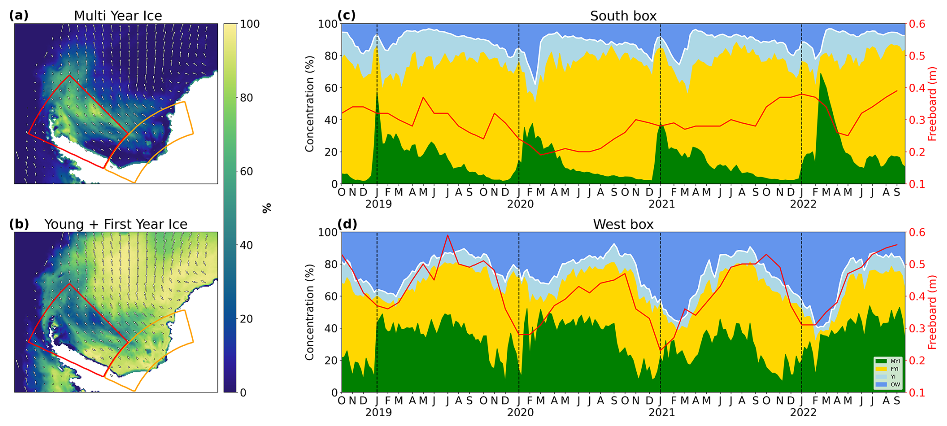
Figure 2 Seasonality of sea ice types in the perennial ice pack. (a, b). Sea ice concentration for (a) MYI and (b) YI + FYI in the Weddell Sea averaged between June–August 2019, with concurrent sea ice drift vectors (Melsheimer et al., 2023; Tschudi et al., 2019). The orange and red boxes in each panel delimit the southern and western regions, respectively. (c, d) Weekly resolved time series of sea ice types averaged over the southern (c) and western (d) regions. The white line highlights the total sea ice concentration. The red line represents the area-weighted sea ice freeboard thickness at monthly resolution obtained from ICESat-2's gridded product (ATL20).

The FCD is defined as the count of individual floes binned over their respective chord lengths (Fig. 3a). Aggregated over the full study period (October 2018–October 2022), and over each region separately, the FCD displays a monotonic decline with chord length between approximately 70 m and 10 km. This distribution can be interpreted as a higher proportion of small floes relative to larger ones. We fit the FCD using a power law with exponent α_FCD between chord lengths spanning 100 m to 10 km and a uniform bin size of 50 m. We find that ${\mathit{\alpha }}_{\text{FCD}}=-\mathrm{1.2}$ in both regions.

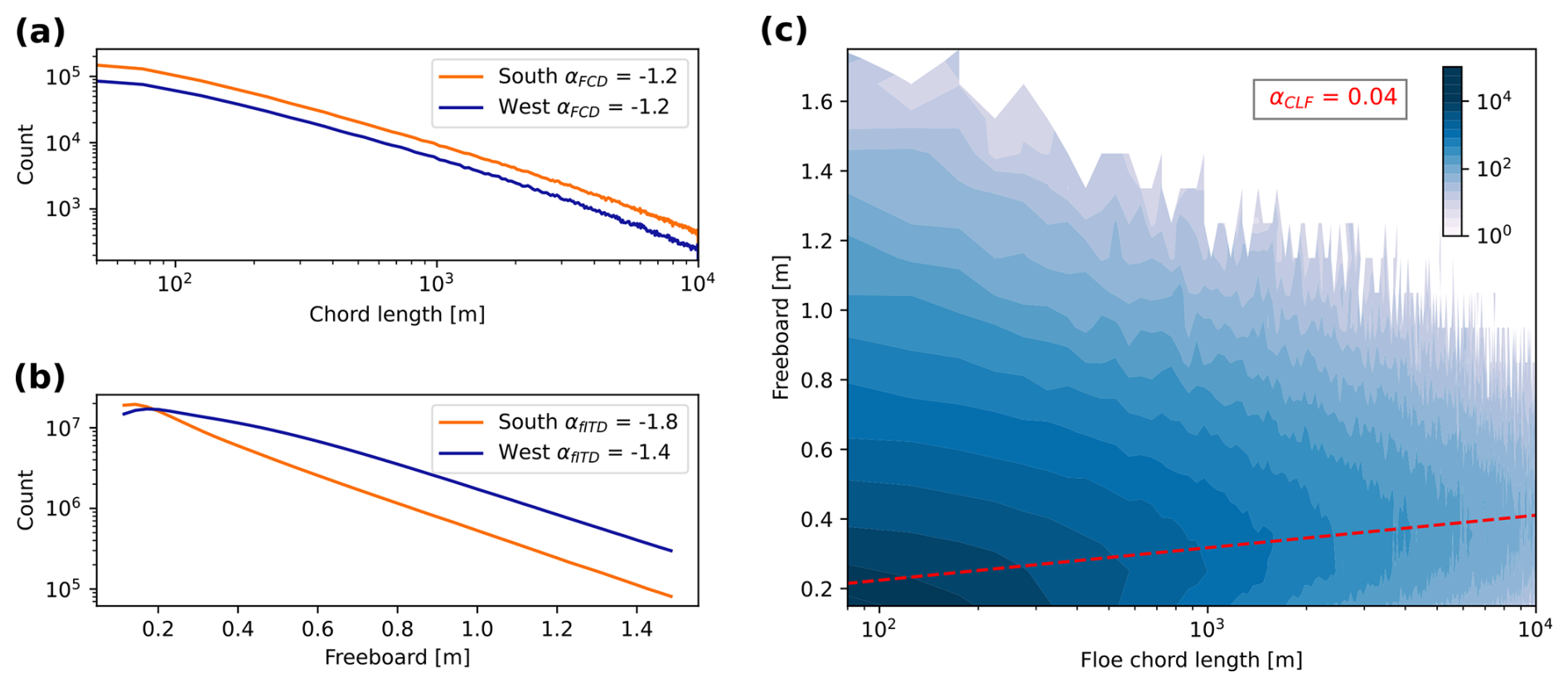
Figure 3 Floe-scale properties aggregated over all the ICESat-2 data collected between October 2018 and October 2022. (a) FCD evaluated over a 50 m bin size and (b) fITD evaluated over a 0.02 m bin size for the southern (orange) and western regions (blue), respectively. The best-fit slope for each curve is indicated in the legend (α_FCD and α_fITD, respectively). (c) Joint floe chord and freeboard thickness distribution showing the number of floes counted over the same bin ranges as in (a) and (b). The dotted red line marks the mean freeboard value over the chord length range and has a slope of α_CLF=0.04 on this graph. The variability across seasons, regions, and individual floes is shown in Fig. A4.

The fITD is evaluated as the count of individual ICESat-2 segments binned over their respective freeboard thickness (Fig. 3b). The distribution declines mostly monotonically over these bin sizes, which signifies a larger proportion of thin segments relative to thicker ones, except for a small fITD peak around 0.2 m in both regions. We approximate the fITD as an exponential curve with a coefficient α_fITD between 0.2 and 1.5 m and a bin size of 0.02 m. The fITD slope is relatively steep in the southern box (${\mathit{\alpha }}_{\text{fITD}}=-\mathrm{1.7}$) and shallower in the western box (${\mathit{\alpha }}_{\text{fITD}}=-\mathrm{1.4}$), reflecting the presence of thicker ice near the Antarctic Peninsula.

We evaluate the joint chord length and freeboard thickness distribution using the same bin sizes as for the individual distributions (Fig. 3c). The contours of the joint distribution have a parabolic shape such that small and thin floes significantly outnumber thick and large ones (Fig. 3c). Very high freeboard values (>1 m) are also observed over small floe lengths, which may reflect the presence of icebergs or broken landfast ice (Sect. 2.3).

The peak of each contour of the joint distribution represents the freeboard thickness of the majority of floes within a given floe chord length range. These peaks coincide with the mean freeboard thickness evaluated over that range, which is depicted by the dotted red line. The mean freeboard thickness is well represented by a fit of the form $h\propto {\mathit{\alpha }}_{\text{CLF}}\cdot \log \left(x\right)$, where x is the chord length. We find α_CLF=0.04 such that, on average, larger floes have a greater freeboard thickness than smaller floes. This conclusion also holds during individual seasons and for both regions, though there is substantial variability among individual floes (Fig. A4). We note that while the mean floe thickness is positively correlated with the mean floe chord length, this correlation is negative for thicker floes, as shown by the downward-sloping contours of the joint distribution for large freeboard values.

We investigate the variability of the FCD and fITD by evaluating these quantities over subsamples of the total 4-year data period. We choose to study a characteristic seasonal cycle by detrending and compositing the anomaly in the slope of these distributions. We evaluate α_FCD,α_fITD, and α_CLF in chunks of 3 d for the two regions separately, calculate the time series of the anomaly relative to the detrended annual mean, and composite the results over a seasonal cycle. The final time series is smoothed using a periodic Gaussian filter with a window of 6 d. We find that the seasonality of the slopes is not very sensitive to the number of chunks (between 2 and 10 d) or the various lead definitions considered in this work (Fig. A2).

The southern and western regions of the pack display a consistent seasonal evolution in their FCD slope anomaly ${\mathit{\alpha }}_{\text{FCD}}^{\prime }$ (Fig. 4a). Around November, at the start of the melt season, ${\mathit{\alpha }}_{\text{FCD}}^{\prime }$ is positive, which represents a higher proportion of larger floes relative to the annual mean. Throughout the melt season, between November and February, ${\mathit{\alpha }}_{\text{FCD}}^{\prime }$ decreases and becomes negative around December as a result of the pack fracturing into increasingly small floes. From February to October, ${\mathit{\alpha }}_{\text{FCD}}^{\prime }$ increases and becomes positive again around April, as sea ice refreezes into a more consolidated pack composed of larger floes. Despite some variability, ${\mathit{\alpha }}_{\text{FCD}}^{\prime }$ is statistically different from zero for a substantial portion of the year in both regions.

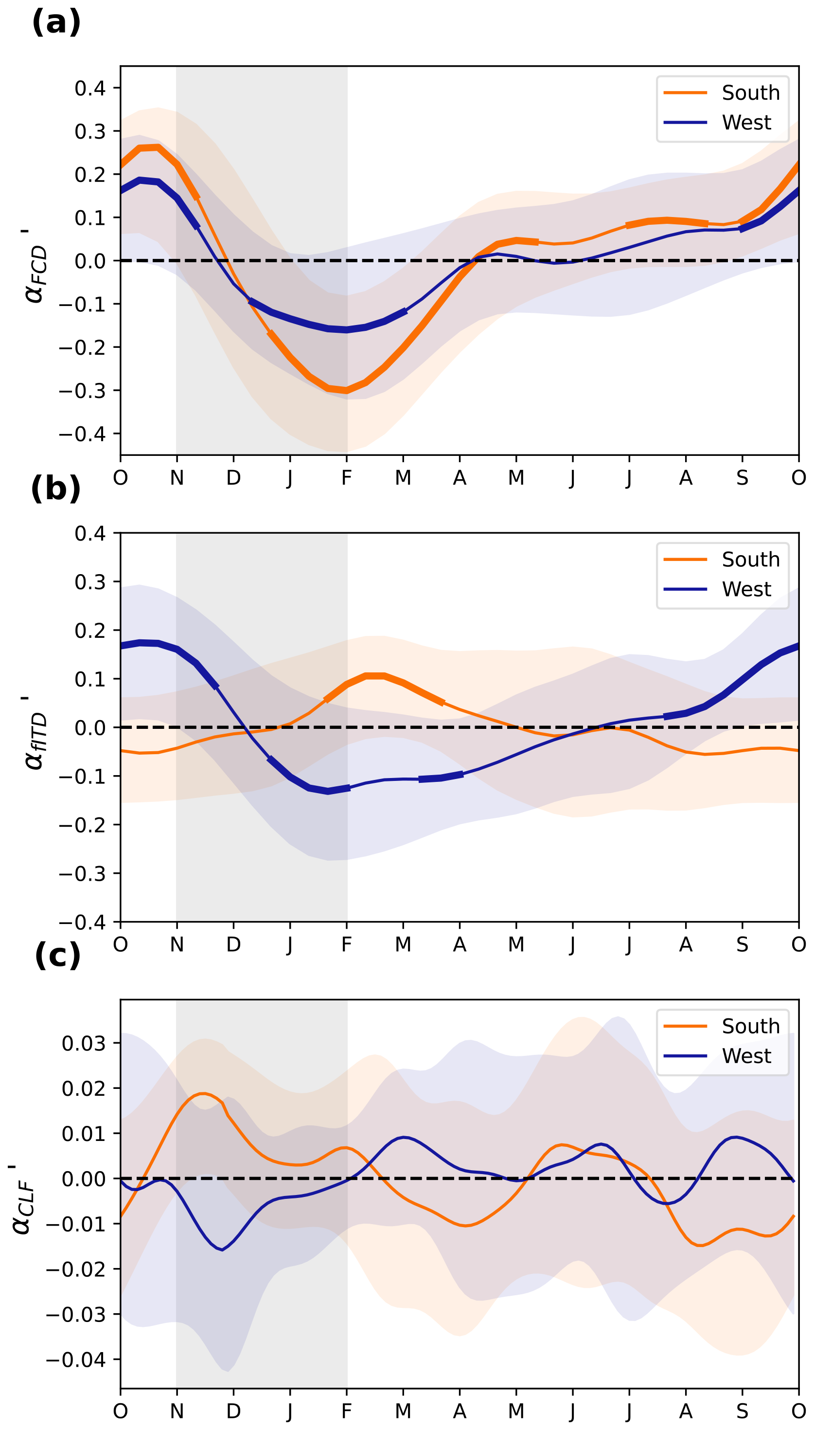
Figure 4 (a) FCD slope anomaly (${\mathit{\alpha }}_{\text{FCD}}^{\prime }$: power law) composited over a seasonal cycle and smoothed by a periodic Gaussian filter with a window of 6 d. Positive values of ${\mathit{\alpha }}_{\text{FCD}}^{\prime }$ signify a reduced proportion of small floes relative to the annual mean. The colored shading represents 2 standard deviations of variability over the 4 years considered, and the bold parts of the curve represent times during which ${\mathit{\alpha }}_{\text{FCD}}^{\prime }$ is significantly different from zero based on a p value of 0.05. The vertical gray shading highlights the approximate duration of sea ice melt, as inferred from Fig. 2. (b) As in (a) but for the fITD slope anomaly (${\mathit{\alpha }}_{\text{fITD}}^{\prime }$: exponential), where a positive anomaly signifies a reduced proportion of thin floes relative to the annual mean. (c) As in (a) but for the correlation between mean floe chord length and freeboard thickness (${\mathit{\alpha }}_{\text{CLF}}^{\prime }$: logarithmic), where a positive anomaly signifies an increased positive correlation relative to the annual mean.

Unlike the FCD, the seasonality of the fITD slope is not consistently in phase between the southern and western regions of the sea ice cover (Fig. 4b). In the west, ${\mathit{\alpha }}_{\text{fITD}}^{\prime }$ is positive at the start of the melt season, which signifies a higher proportion of thick ice segments relative to the annual mean. During the melt season, between November and February, ${\mathit{\alpha }}_{\text{fITD}}^{\prime }$ declines and becomes negative around December such that the proportion of thicker ice becomes smaller than the annual mean. Between February and October, ${\mathit{\alpha }}_{\text{fITD}}^{\prime }$ increases and becomes positive again around June. Despite some variability, ${\mathit{\alpha }}_{\text{fITD}}^{\prime }$ is statistically different from zero for a sizable portion of the year in the west. In the south, around November, ${\mathit{\alpha }}_{\text{fITD}}^{\prime }$ is slightly negative. During the melt season, between November and February, ${\mathit{\alpha }}_{\text{fITD}}^{\prime }$ increases and becomes positive around January such that the proportion of thicker floes becomes greater than in the annual mean. During the freezing season, between February and October, ${\mathit{\alpha }}_{\text{fITD}}^{\prime }$ declines and reaches slightly negative values. However, the variability is large in the south, and the fITD signal is not statistically significant, except between mid-January and April.

The correlation slope between mean freeboard thickness and mean floe chord length (α_CLF; dotted red line in Fig. 3c) also varies seasonally (Fig. 4c). The magnitude of these fluctuations is of the same order as the annual mean signal such that the sign of the correlation remains positive throughout the year, as seen over individual seasons (Fig. A4). As with ${\mathit{\alpha }}_{\text{fITD}}^{\prime }$, the composited mean seasonal fluctuations in ${\mathit{\alpha }}_{\text{CLF}}^{\prime }$ are generally mirrored between the southern and western regions. However, the variability is large and the seasonal signal in ${\mathit{\alpha }}_{\text{CLF}}^{\prime }$ is not statistically significant over any part of the year.

3.3 Lead width and spacing

The size and thickness of floes are influenced by the width and spacing between sea ice leads, which provide large heat exchanges with the ocean and atmosphere, as well as space for inter-floe collisions (Maykut and Perovich, 1987). We investigate the LWD by binning leads according to their width, which is defined as the distance between the first and last contiguous segments identified as a lead along a track. As with the FCD, we focus on the dark and specular leads identified by the ATL07 algorithm and report on the sensitivity of our results to the lead definition in Figs. A2 and A3.

We evaluate the LWD by aggregating the leads identified over the 4 years of data in bins with lead widths ranging between 30 m and 3 km. The LWD is almost identical for the southern and western regions of the pack, characterized by a mostly monotonic decrease with size, which represents a larger proportion of narrow leads compared to wide leads (Fig. 5a). The variability in the LWD for lead widths greater than 700 m is caused by their relatively small count (<10). For statistical significance, we do not take account of these wide leads in our subsequent analysis. The mean slope of the LWD evaluated between 20 and 700 m is α_LWD = −3.1 for both regions, which is substantially steeper than α_FCD (Fig. 3a).

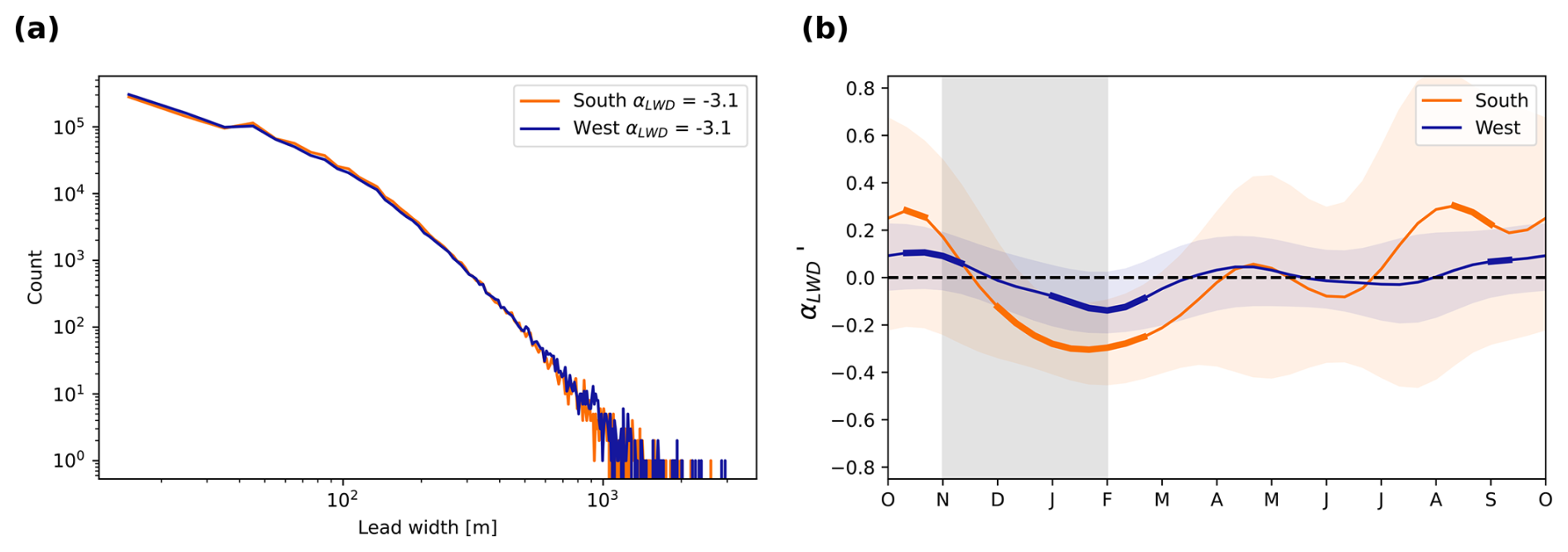
Figure 5 (a) LWD for the southern (orange) and western (blue) regions evaluated over a bin size of 10 m. (b) As in Fig. 4 but for the LWD slope anomaly (${\mathit{\alpha }}_{\text{LWD}}^{\prime }$: power law). Positive values of ${\mathit{\alpha }}_{\text{LWD}}^{\prime }$ signify an increased proportion of wider leads relative to the annual mean.

Following the method used to produce the panels in Fig. 4, we evaluate the seasonal composite of the LWD slope anomaly ${\mathit{\alpha }}_{\text{LWD}}^{\prime }$ in Fig. 5b. Over both regions, ${\mathit{\alpha }}_{\text{LWD}}^{\prime }$ tends to be positive in October, which represents a larger fraction of wide leads relative to the annual mean. During the melt season, ${\mathit{\alpha }}_{\text{LWD}}^{\prime }$ declines and becomes negative, representing a larger fraction of narrow leads relative to the annual mean. The LWD then progressively increases back to its October distribution over the course of the freezing period. The seasonal signal in ${\mathit{\alpha }}_{\text{LWD}}^{\prime }$ is only statistically significant during parts of the melt season and toward the end of the freezing period. The magnitude of the anomalies tends to be larger in the south compared to the west. While there may be differences in the phasing of the signal between the two regions, those are difficult to evaluate due to large variability among the 4 years considered. Different lead definitions also give a different magnitude and phasing in the seasonality of the LWD, though broadly ${\mathit{\alpha }}_{\text{LWD}}^{\prime }$ tends to be negative between December and February and positive between May and July (Fig. A2).

The spacing between leads can also be a useful metric for describing the compactness of the sea ice cover and its potential response to atmospheric forcings and surface heat fluxes. Here, we define the lead spacings as the distances between all the leads along a given track that have a width within a given bin size category. We then average the lead spacings across all the tracks within a given region to produce the mean lead spacing as a function of lead width (Fig. 6). We do not examine the spacing between leads wider than 300 m, as they do not occur frequently enough to provide robust statistics (Fig. 5a). In the annual mean, the average spacing between leads contained within the 50 m width bin size category is approximately 20 km for both regions. In the west, the mean lead spacing increases to a maximum of 102 km for 180 m wide leads, while in the south the mean lead spacing increases to a maximum of 41 km for 150 m wide leads. The lead spacing curves subsequently flatten out around their respective maxima in both regions. Consequently, the mean lead spacing is up to 2.5 times larger in the west compared to the south, despite these two regions having the same α_LWD and α_FCD.

Figure 6 Mean lead spacing computed at each lead width bin category between 30–300 m with a constant bin spacing of 10 m for the (a) western and (b) southern regions. The colored scatter points represent aggregates for selected months, while the black “cross” symbols represent yearly mean aggregates.

The relationship between lead spacing and lead width becomes less clear with lead widths increasing from the maximum lead spacing. For example, beyond lead widths of 200 m in the western region, the curve becomes increasingly interrupted. Though the maxima of each curve here occurs at a different lead width, there is a similar breakdown of the relationship as lead width increases beyond the maximum lead spacing. This is also the case with different lead definitions (Fig. A3). Thus, there appears to be a limit to how large a lead width can be while still having a discernible relationship with lead spacing.

We probe the seasonality of the lead spacing by aggregating data for individual months across the 4-year data period (Fig. 6). In both regions, the broad shape of the lead spacing distribution is similar to the annual mean but with varying magnitudes. In the west, from July to January, the mean spacing between leads decreases across all lead width categories, reflecting a more fractured sea ice cover by the end of the melt season, before increasing again between April and July. In the south, the seasonality in mean lead spacing is less pronounced. Narrow leads (<120 m) follow a similar phasing as in the west, while wider leads (>120 m) have larger mean spacing in the summer compared to the winter. Characterizing leads using a freeboard threshold instead of the identification provided by ICESat-2 can reduce the seasonality in the lead width spacing signal (Fig. A3). This may be due to the misidentification of thin ice as leads, especially near areas of widely distributed thin ice (Koo et al., 2023). Nevertheless, the seasonal trend in lead width spacing remains consistent across lead definitions.

3.4 Vertical floe roundness

The ICESat-2 along-track freeboard data can be used to investigate the shape of floes in the vertical direction and their associated changes over the seasonal cycle. We quantify the characteristic vertical profile of floes by compositing their freeboard thickness along their respective chord lengths. The floes are grouped into the following three size categories for the compositing process: small (100–500 m), medium (500 m–5 km), and large (5–50 km). Composites are produced by averaging the freeboard thickness over half the normalized floe chord distance such that the resulting average represents the mean floe profile from the floe edge to the middle of the chord length. Both halves of a given floe chord are weighed equally and considered independently in the compositing procedure.

The vertical profiles of freeboard thickness averaged over all floes reveal a semi-dome shape for all three size categories (Fig. 7a) such that floes on average have a smaller freeboard at their edges compared to their chord centers. The standard deviation around these mean profiles is substantial, reflecting the large freeboard variability along the surface of individual floes (Fig. 1). Consistent with inferences obtained from the joint chord and freeboard thickness distribution (Fig. 3c), the mean composited profiles show that larger floes have a greater overall freeboard thickness than smaller floes.

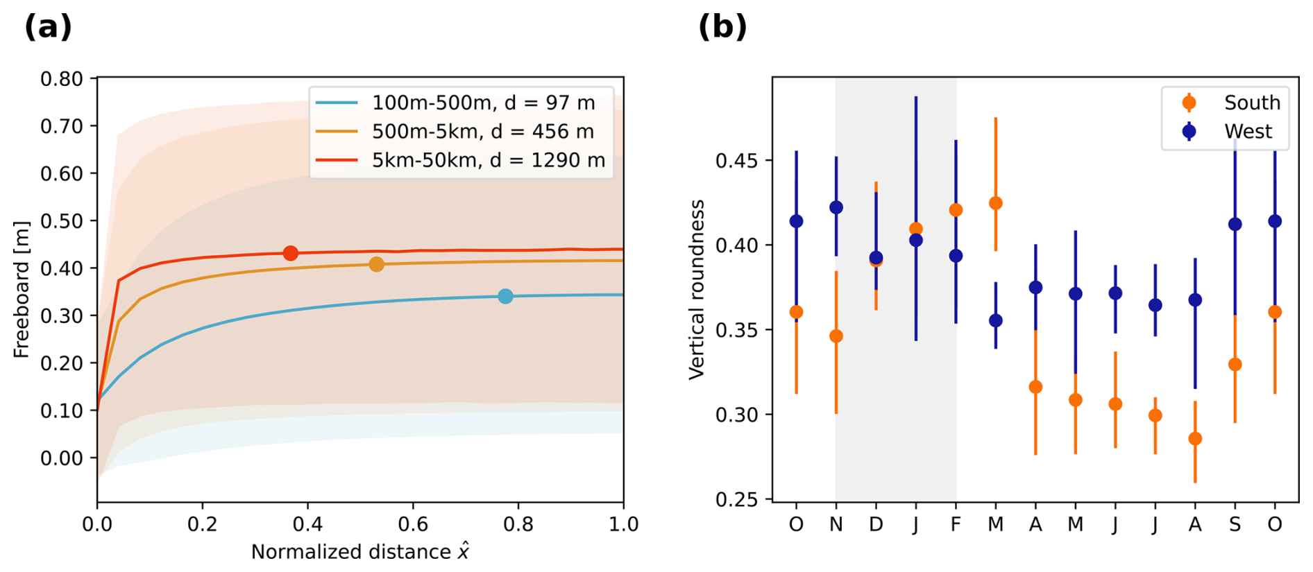
Figure 7 (a) Composited vertical floe profiles obtained by averaging the freeboard distribution along each floe chord and over a normalized horizontal distance $\widehat{x}$. We consider all the floes detected within the analysis period and over both regions. The compositing is done separately for small (100–500 m, blue), medium (500 m–5 km, orange), and large (5–50 km, red) floes, with each category comprising 2.8 $\times {\mathrm{10}}^{\mathrm{5}},\mathrm{3.6}\times {\mathrm{10}}^{\mathrm{5}}$, and 1.5 ×10⁵ floes, respectively. The shading represents 2 standard deviations of variability across individual floes. The colored dots represent the distance d over which the profiles flatten, defined as the point along $\widehat{x}$ where the profile slope drops below 0.05 in normalized units. (b) Monthly mean vertical roundness of floes for the southern (orange) and western (blue) regions calculated from floe profiles including all sizes (100 m–50 km). The error bars represent the minimum to maximum ranges of vertical roundness reported for the 4 years of analysis. The vertical gray shading highlights the approximate duration of the sea ice melt period.

The mean vertical shape of floes may be a useful indicator of surface processes occurring at their respective scales. To characterize these floe shapes, we evaluate the distance d over which the composited profiles become flat based on a slope threshold of 0.05 in normalized units. The distance d is 97 m for small floes, 456 m for medium floes, and 1.3 km for large floes or 0.78, 0.57, and 0.36, respectively, in normalized units. The accuracy of these d values may be affected by the altimeter footprint (∼11–26 m), but this error is expected to diminish with the compositing procedure.

We further quantify the vertical roundness of floes α_vr by integrating under the curve of the mean floe profiles and normalizing by the area of a rectangle enclosing the profile, as follows:

$$\begin{array}{}\text{(1)}& {\displaystyle }{\displaystyle }{\mathit{\alpha }}_{\text{vr}}=\mathrm{1}-{\displaystyle \frac{{\int }_{\mathrm{0}}^{\mathrm{1}}\widehat{p}\left(\widehat{x}\right)\mathrm{d}\widehat{x}-\mathit{\pi }/\mathrm{4}}{\mathrm{1}-\mathit{\pi }/\mathrm{4}}},\end{array}$$

where $\widehat{x}$ is the normalized distance along a floe chord and $\widehat{p}\left(\widehat{x}\right)$ is the corresponding freeboard height profile along the floe. A perfectly round profile has α_vr=1, while a square profile tends to α_vr=0. In the annual mean, α_vr is 0.76 for small floes, 0.37 for medium floes, and 0.21 for large floes. The smallest floes are thus 3.6 times rounder than the largest floes on average.

In both regions, α_vr averaged across all floes varies over the seasonal cycle. In the south, α_vr tends to increase between August and February, before dropping sharply between March and April, at the start of the freezing cycle (Fig. 7b). In the west, α_vr increases between August and September, but the variability over the 4 years considered is too large to conclusively report on the rest of the seasonal cycle. In both regions, α_vr averaged over individual size categories does not vary significantly throughout the year (not shown), which means that the seasonal variability in the mean vertical roundness across all sizes is driven by changes in the size and freeboard thickness distribution of floes. The increase in α_vr during spring and summer is thus likely linked to the proliferation of smaller floes with rounder profiles. The timing of the seasonal cycle in α_vr is not highly sensitive to the different floe definitions considered in this work (not shown).

4 Discussion

The spatial patterns in sea ice types show that the western portion of the Weddell Sea is composed of thicker and older sea ice than in the southern region (Sect. 3.1), which is consistent with past inferences (Haas et al., 2008; Kacimi and Kwok, 2020; Melsheimer et al., 2023). The annual mean sea ice concentration is also lower in the western region due to summer melt and northward export toward the ACC. In spite of these regional differences, the seasonality of the FCD is consistent between the western and southern portions of the pack and is in phase with the asymmetric melt–freeze cycle over the perennial sea ice pack (Sect. 3.2). The spatial homogeneity in FCD suggests that it is not strongly sensitive to localized differences in environmental conditions but may instead be controlled by processes occurring at larger scales. While the processes responsible for the asymmetry in the melt–freeze cycle remain to be fully understood (Roach et al., 2022; Goosse et al., 2023), our results suggest that its phasing plays a first-order role in governing the seasonality of the FCD.

In contrast to the FCD, the freeboard fITD displays notable differences between the southern and western parts of the Weddell Sea (Fig. 4). In the annual mean, there is a greater fraction of thicker freeboard segments in the west, likely due to strong compaction against the Antarctic Peninsula (Yi et al., 2011). During the melt season, while the total freeboard thickness decreases in both regions (Fig. 2c and d), the fraction of thicker ice segments increases in the south and decreases in the west (Fig. 4b). The diminishing fraction of thick ice in the west is consistent with the observed advection of MYI away from the Antarctic Peninsula (Fig. 2a) and potentially reduced compaction due to looser sea ice concentration. In the south, the increasing fraction of thick ice in summer may instead be caused by the preferential melt of thin ice in response to solar forcing or changes in the import of younger ice from the east. Seasonal changes in the freeboard thickness may also be modulated by snowfall, whose effect cannot be parsed from ICESat-2 data alone. At coarse scales, previous studies have employed linear relationships between the snow depth and freeboard (Kacimi and Kwok, 2020; Kurtz and Markus, 2012; Xie et al., 2011; Worby et al., 2008), but further observational is required to assess the relationship between the ITD and fITD at fine scales (Arndt, 2022).

Metrics pertaining to sea ice leads provide additional information on the spatial structure of the pack. As with the FCD, the LWD has a similar shape in the western and southern portions of the Weddell Sea (Fig. 5a). On the other hand, the mean lead spacing, when calculated within individual lead width categories, is higher in the west by a factor of up to 2.5 relative to the south (Fig. 6). This mean lead spacing is not necessarily equivalent to the mean floe size, as it additionally depends on the sea ice concentration, which differs between the two regions, and the ordering of individual leads along a track. The larger lead spacing in the western region is consistent with a more compacted pack due to sea ice impinging upon the Antarctic Peninsula. The seasonal change in the lead spacing also coincides with increased compaction, producing more sparsely distributed leads in the winter and the opposite in the summer.

Throughout the seasonal cycle, the joint chord–freeboard distribution displays a positive correlation between the mean floe chord length and the mean floe freeboard (Figs. 3 and 4c). Processes such as snow export into leads (Leonard and Maksym, 2011; Moon et al., 2019), flooding (Ackley et al., 2020; Yi et al., 2011), and the formation of thin nilas at floe edges (Farrell et al., 2020) may contribute to this positive correlation. The composited vertical shapes of floes show that the characteristic vertical rounding distance d increases with floe size (Fig. 7), which suggests that different erosive mechanisms may dominate at different spatial scales. Retrievals over thin ice are also more likely to be misclassified as open water, which could lead to a spurious correlation between lateral floe size and freeboard thickness. Nevertheless, this correlation exists for all the lead detection schemes considered here.

Inferring sea ice properties with ICESat-2 is subject to several caveats. The use of along-track altimetry leaves uncertainty about the 2-D distribution of floe sizes, ridges, and leads (Horvat et al., 2019; Farrell et al., 2020; Koo et al., 2023). Moreover, accurately estimating the location of leads along ICESat-2 tracks is an ongoing challenge, notably for dark leads (Petty et al., 2021). In some cases, leads can be misclassified as sea ice, whereas the opposite may occur in others. While quantitative estimates of the FCD, LWD, and floe roundness vary with the different lead definitions considered in this work, our general conclusions are robust to this choice. Furthermore, our use of a single slope to characterize the seasonal evolution of the FCD, fITD, and LWD distributions can blur potentially different mechanisms occurring across a wide range of scales. Future work may benefit from considering alternative approximations of these distributions to explore more detailed and localized processes (Montiel and Mokus, 2022). ICESat-2 freeboard estimates also do not allow us to parse the contributions of snow vs. ice, which limits our ability to understand the mechanisms responsible for the observed seasonality in fITD and floe roundness. Conducting floe-scale analyses using a snow-penetrating altimeter could be a useful extension to this work.

5 Conclusions

This study uses various satellite products, including along-track altimetry from ICESat-2, to explore the seasonality of the perennial sea ice pack in the Weddell Sea. We contrast the behavior of the western portion of the pack, characterized by a high fraction of MYI, with the southern region, which is largely composed of FYI. Despite different sea ice types, the seasonality of the floe chord distribution, a proxy for the floe size distribution, is consistent between the two regions. On the other hand, the evolution of the freeboard ice thickness distribution suggests an antiphase relationship between the two regions during the melt period, potentially due to the differential effects of thermodynamics vs. dynamics in governing the seasonal cycle.

The mean vertical freeboard of floes exhibits a dome-shaped profile, characterized by thinner ice at the floe edge and thicker ice toward its center. Composited profiles show that larger floes tend to be thicker and more vertically square than smaller floes. The proliferation of smaller and vertically rounder floes in the summer causes an increase in the mean vertical roundness in the southern portion of the sea ice pack. The mean spacing between leads is smaller in the west compared to the south, which is consistent with a more compact sea ice cover in the west, likely due to compaction against the Antarctic Peninsula (Kacimi and Kwok, 2020).

Feedbacks linking basin to floe-scale processes are not resolved in most climate models and may in part explain biases in modeled sea ice trends. The sea ice metrics considered here may help calibrate floe-resolving models (Herman, 2016; Manucharyan and Montemuro, 2022; Moncada et al., 2023) and facilitate the development of subgrid parameterizations designed for continuum-based sea ice models (Roach et al., 2018; Boutin et al., 2020). The roundness of the dome-shaped vertical profiles exhibited by floes may notably assist in parameterizing lateral erosive processes, which play an important role in shaping the joint floe chord and freeboard thickness distribution. The freeboard thickness profiles may help examine the effects of lateral melt (Horvat et al., 2016; Gupta and Thompson, 2022), flooding (Ackley et al., 2020), and snow export (Leonard and Maksym, 2011; Moon et al., 2019), though disentangling their relative importance requires independent estimates of snow and ice thickness over individual floes. A comparison of such observed metrics with results from floe-aware models could nevertheless provide a useful diagnostic of model performance and opportunities for data assimilation (Sievers et al., 2023).

As basin-wide forcings continue to change around Antarctica, austral sea ice may transition toward a pack composed of smaller and thinner floes that are more susceptible to drift and melt. Evidence for a younger, thinner, and more mobile sea ice cover has been reported in the Arctic Ocean (Rampal et al., 2009; Notz and Stroeve, 2016; Mallett et al., 2021), while Antarctica has experienced several recent episodes of rapid sea ice loss, suggesting a potential regime shift towards a longer-term decline (Turner et al., 2022; Purich and Doddridge, 2023). Finely resolved inferences on the winter to summer transition of the pack, such as the ones presented in this work, may help improve our understanding of longer-term warming trends and parse their regional differences more precisely.

Appendix A

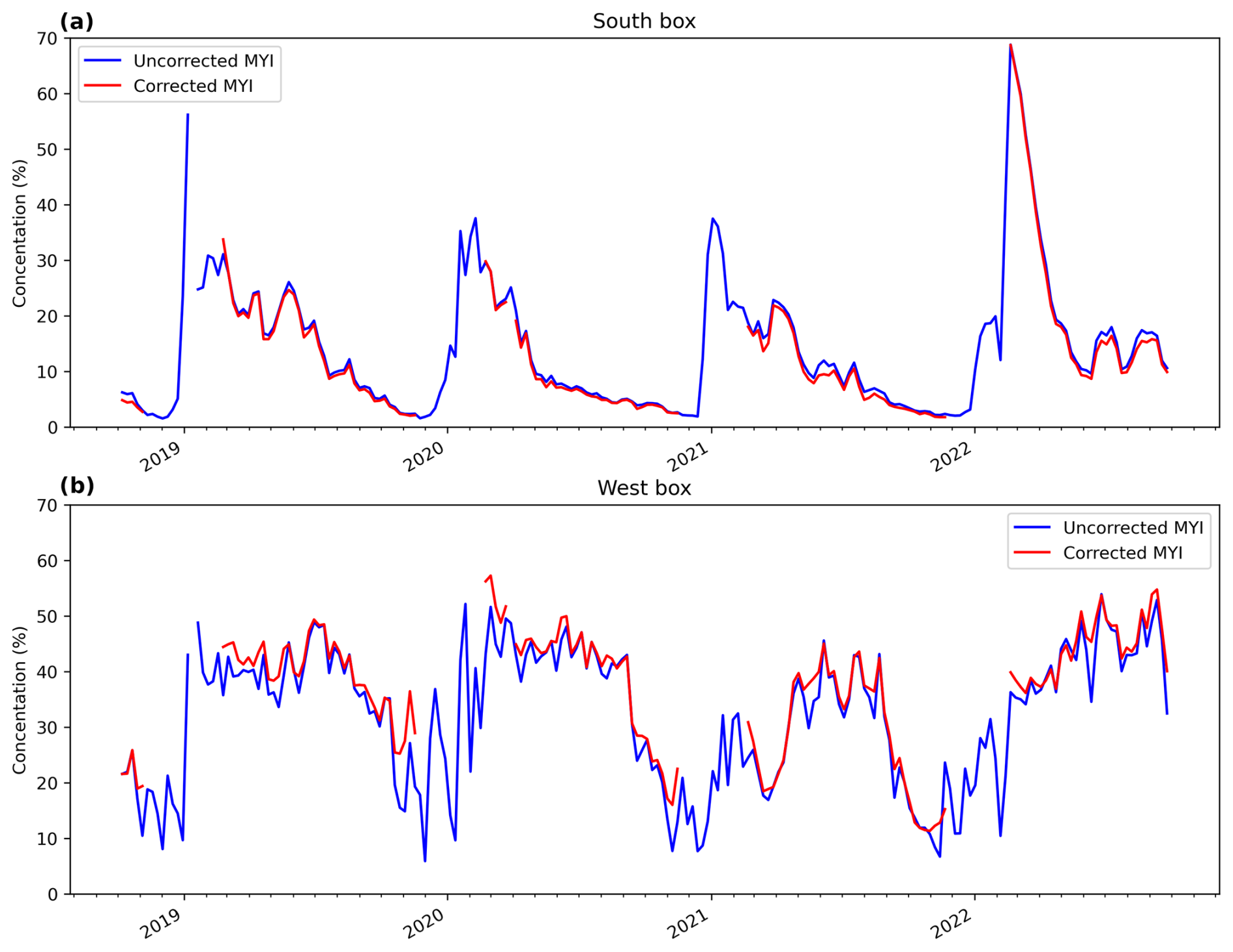
Figure A1 Comparison between the corrected and uncorrected versions of the MYI product averaged over the (a) southern and (b) western regions.

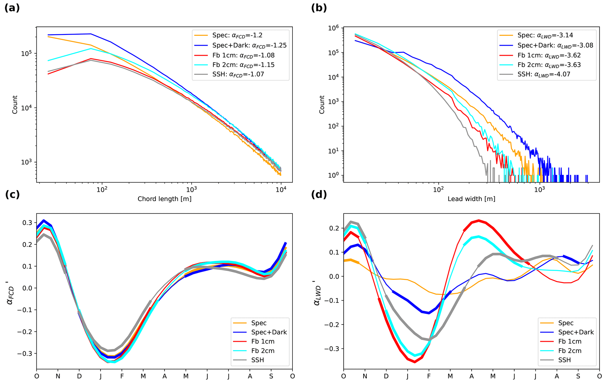
Figure A2 Sensitivity of the FCD and LWD to the lead detection method. (a) FCD for all floe chords and (b) LWD for all leads. (c, d) Seasonal composites of (c) ${\mathit{\alpha }}_{\text{FCD}}^{\prime }$ and (d) ${\mathit{\alpha }}_{\text{LWD}}^{\prime }$, calculated as in Figs. 4a and 5b, respectively, combining the southern and western regions. The following lead detection methods are considered: specular, specular + dark, freeboard height threshold at 1 cm, freeboard height threshold at 2 cm, and SSH flag. The thicker parts of each curve are significantly different from zero based on a p value of 0.05.

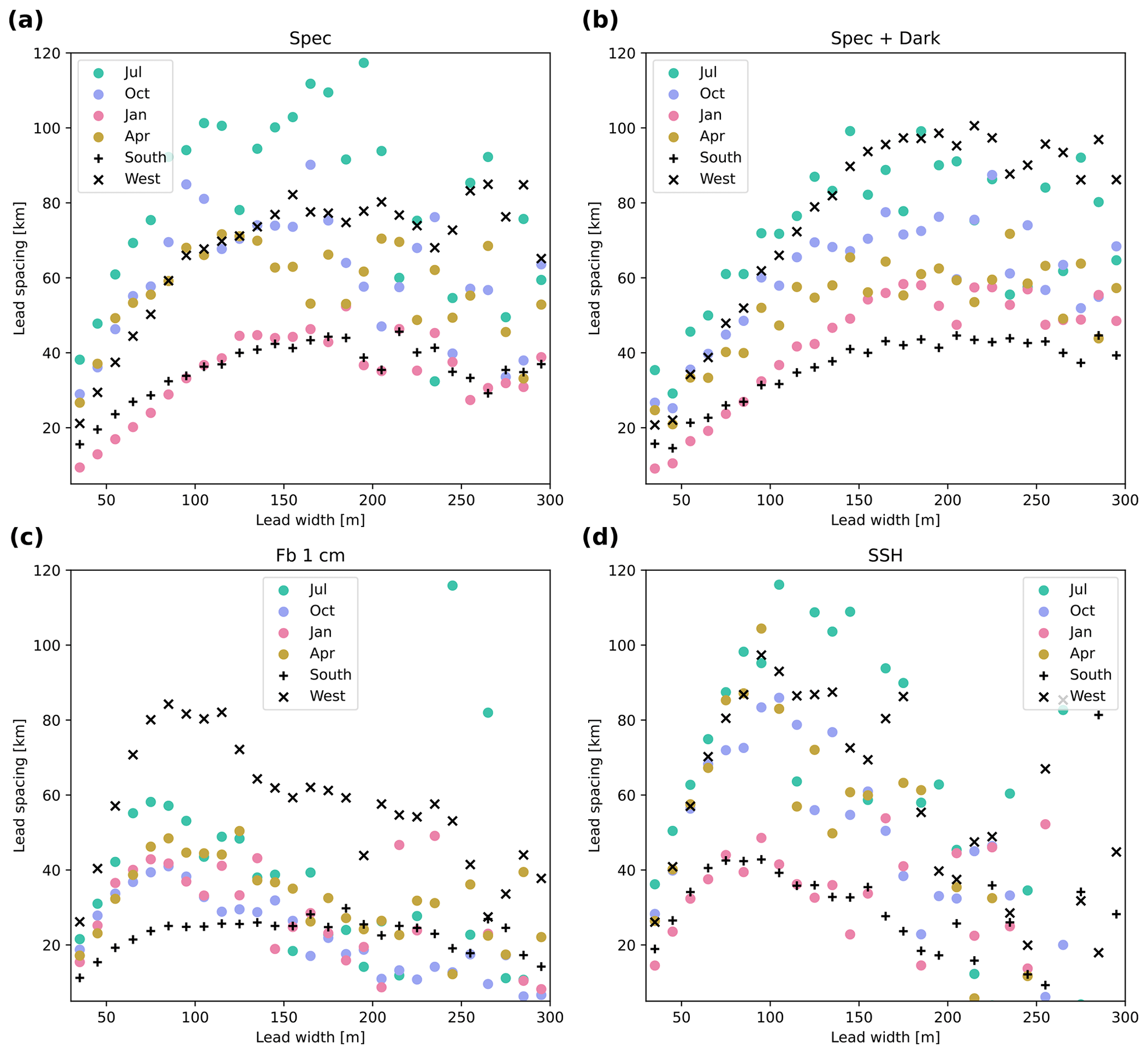
Figure A3 Sensitivity of the lead spacing combining the southern and western regions for the following lead definitions: (a) specular, (b) specular + dark, (c) freeboard height threshold at 1 cm, and (d) SSH flag. The analysis is conducted as in Fig. 6.

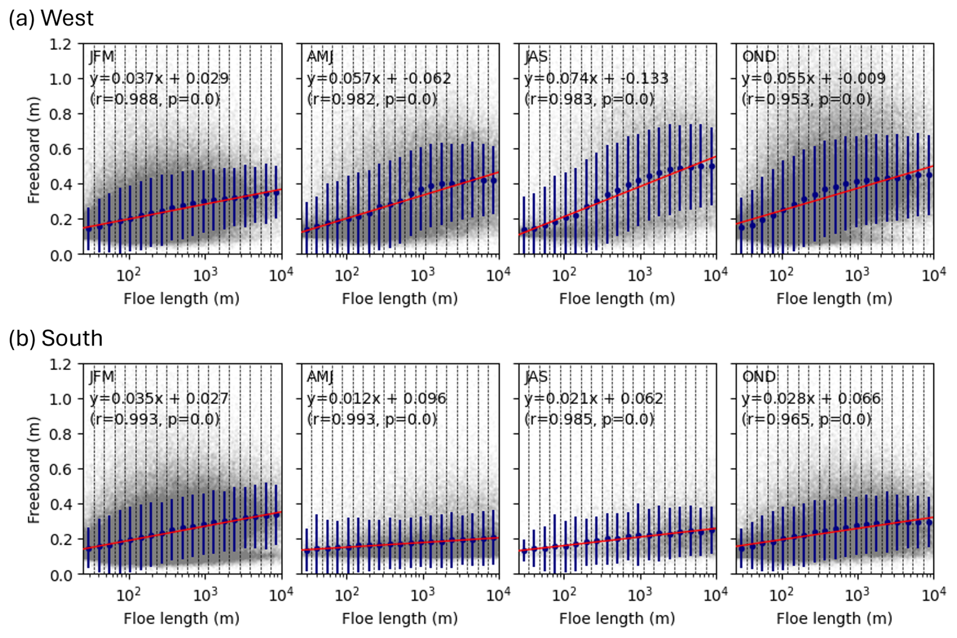
Figure A4 Mean floe freeboard vs. floe chord length aggregated in four seasons during the years 2019–2022 for the (a) western and (b) southern regions of the pack. The floe chord length is divided into 20 bins on a log scale. The gray points show individual floes. The red line indicates the linear best-fit line and its corresponding statistics are detailed in each panel. The navy dots represent the median freeboard for each bin range, and the vertical navy bar indicates the standard deviation of the freeboard.