Bathymetry-constrained impact of relative sea-level change on basal melting in Antarctica

Relative sea level (local water depth) on the Antarctic continent is changing through the complex interplay of processes associated with glacial isostatic adjustment (GIA). This involves near-field viscoelastic bedrock displacement and gravitational effects in response to changes in Antarctic ice load but also far-field interhemispheric effects on the sea-level pattern. On glacial timescales, these changes can be of the order of several hundred meters, potentially affecting the access of ocean water masses at different depths to Antarctic grounding lines and ice-sheet margins. Due to strong vertical gradients in ocean temperature and salinity at the continental-shelf margin, basal melt rates of ice shelves have the potential to change just by variations in relative sea level alone. Based on simulated relative sea-level change from coupled ice-sheet–GIA model experiments and the analysis of topographic features such as troughs and sills that regulate the access of open-ocean water masses onto the continental shelf, we derive maximum estimates of Antarctic basal melt rate changes, solely driven by relative sea-level variations. Our results suggest that the effect of relative sea-level changes on basal melting is limited, especially compared to transient changes in the climate forcing.

1 Introduction

Global-mean sea level (GMSL) varies on glacial–interglacial timescales of the order of 100 m. The dominant component of GMSL changes since the Last Glacial Maximum (LGM, ca. 21 000 years before present (kyr BP); Gebbie, 2020) is determined by the mass redistribution between ocean and land (e.g., by ice-sheet changes; Miller et al., 2020; Horwath et al., 2022), which is referred to as barystatic sea-level change (Gregory et al., 2019). Changes in ocean density (steric effects) play only a minor role on glacial timescales but have a relevant contribution to anthropogenic sea-level rise (Gebbie, 2020; Marcos and Amores, 2014). The global distribution of sea level follows an equipotential surface, also called the geoid (Gregory et al., 2019), which is determined by the gravity field of ice, water, and the Earth's mantle material, with a feedback on Earth's rotation (Mitrovica et al., 2005). Variations in sea-level height through ocean currents and winds are not included in the geoid definition. The relative sea level (RSL) is the depth of the water column, hence the vertical distance between the geoid and the ocean bathymetry (or when negative, the land surface elevation above the geoid), and it can change through several processes:

1. Changes in ice masses affect the volume and area of the global ocean, leading to a globally distributed, barystatic shift in the geoid height.

2. The mass redistribution between ice and ocean also affects the Earth's rotational axis such that the global sea-level fingerprint adjusts to the change in centrifugal acceleration.

3. The gravitational force exerted by ice masses on the surrounding ocean masses leads to variations in local geoid height near ice sheets following gains or losses of ice mass.

4. Changes in load have deformational (viscoelastic) effects on the solid Earth, leading to subsidence or uplift of the underlying bedrock topography. Due to the flexure of the lithospheric plate and the viscous flow of upper-mantle material, an increase in ice load would therefore produce an uplift at some distance from the center of the load, yielding a reversed (negative) signal in RSL; this is called a “forebulge”. Depending on the local mantle viscosity and lithosphere thickness, these viscoelastic processes can induce vertical changes of hundreds of meters.

These mechanisms act on different spatial and temporal scales, i.e., almost instantaneous in the case of rotational and gravitational effects, whereas bedrock deformation can take several millennia to unfold. All of the mentioned mechanisms are covered by the glacial isostatic adjustment theory (GIA; Farrell and Clark, 1976; Whitehouse, 2018). Global-mean sea level is also influenced by thermosteric effects through changes in ocean water temperature, but this effect is comparably small on glacial timescales.

During the Last Glacial Maximum, GMSL was about 125–134 m lower than today, mainly due to the presence of large ice sheets in the Northern Hemisphere (Yokoyama et al., 2018; Lambeck et al., 2014). Grounded ice in Antarctica reached close to the continental-shelf break (CSB) in many locations during the LGM (Bentley et al., 2014) and held up to 20 $\mathrm{m}\mathrm{s}.\mathrm{l}.\mathrm{e}.$ (sea level equivalent) more ice, according to the literature review in Albrecht et al. (2020b, their Fig. 11b). Today's configuration of the Antarctic Ice Sheet (AIS) still holds enough ice to raise GMSL by approx. 58 m if melted completely (neglecting isostatic or thermal effects; Morlighem et al., 2020). Considering all land-based ice on Earth, including the Greenland Ice Sheet and mountain glaciers, this number increases to approx. 66 m (IPCC AR6 WG1 Chap. 2.3.3.3; Gulev et al., 2021).

While Antarctic ice mass changes have been small in the Late Holocene (approx. the last 4000 years; Jones et al., 2022), the AIS has been losing mass at an increasing rate in the last decades (Shepherd et al., 2012; Rignot et al., 2019; Otosaka et al., 2023). Due to ongoing atmospheric and oceanic warming, it is projected that Antarctica will lose up to 4.4 m s.l.e. ice volume by 2300 under a high-emission scenario (Seroussi et al., 2024). When considering the long-term stability of the ice sheet, Garbe et al. (2020) find that due to several feedback mechanisms, the AIS is bound to become ice-free at warming greater than 10 °C above pre-industrial levels.

The melting of ice shelves, the floating extensions of the marine ice sheets, is highly sensitive to changes in ocean temperatures on the continental shelf, especially when warm water masses intrude into the ice-shelf cavities at depth (Hellmer et al., 2012; Pritchard et al., 2012; Rintoul et al., 2016). Sub-shelf melt rates are generally highest close to the grounding line, where grounded ice becomes afloat (Rydt and Gudmundsson, 2016). For ice-sheet simulations over long timescales, such as glacial cycles, climatic boundary conditions like ocean and atmospheric temperature have to be parameterized in a robust manner. Albrecht et al. (2020a) use a temperature index method and linear response functions to scale present-day ocean temperature observations on the continental shelf, which is the shallow ocean area surrounding the Antarctic Ice Sheet, with climatic variations derived from ice-core data. For shorter timescales, i.e., end-of-century projections, standalone ice-sheet models are typically forced by the output of climate models (Seroussi et al., 2020).

In order to assess the stability and long-term behavior of ice sheets, interactions with the solid Earth and sea level are relevant, as GIA responses can have major feedbacks with ice dynamics (Whitehouse et al., 2019). Albrecht et al. (2024), for instance, use a globally consistent coupled ice-sheet–GIA model framework and find that ice retreat can be significantly slowed down when isostatic rebound is included, in particular when considering a weak Earth structure with low mantle viscosity and thin lithosphere, as reconstructions suggest for the West Antarctic plate (Barletta et al., 2018; Bagge et al., 2021). Coupled ice-sheet–GIA models exist in different modes of complexity, e.g., with regional setups (Coulon et al., 2021; Zeitz et al., 2022), 1D Earth structure (Pollard et al., 2017; Gomez et al., 2020), or globally in 3D, which are just becoming available, like in Gomez et al. (2018), van Calcar et al. (2023), and Albrecht et al. (2024).

GIA processes also influence ocean dynamics in various ways: Rugenstein et al. (2014) demonstrate that the presence of a forebulge, which raises the Southern Ocean floor by approx. 50 m in response to additional ice loading, can significantly alter ocean velocities, frontal structures, and zonal transport. Wilmes et al. (2017) show that tides are affected by changes in RSL patterns. Tinto et al. (2019) argue that sub-shelf bathymetry controls the oceanic flow beneath the Ross Ice Shelf, which is subject to change due to GIA processes. Motivated by these previous studies, the focus of our analysis is how RSL changes can influence basal melting in ice-shelf cavities.

Temperatures and salinities in the Southern Ocean show a strong dependence with depth: while surface waters are close to the freezing point of seawater (ca. −1.9 °C), temperatures increase at an average rate of +0.5 °C per 100 m in the thermocline layer (approx. upper 600 m) and decrease slowly below to reach about 0 °C at 1800 m (see Fig. S1 in the Supplement). Similarly, ocean salinities increase from about 34.0 psu (practical salinity unit) at the surface to ca. 34.7 psu at 600 m depth and stay rather constant below (see Fig. S2). The thermocline layer is characterized by the transition between cold and fresh surface waters and warmer and saltier Circumpolar Deep Water (CDW). As (positive values of) RSL indicates the local water column depth, positive changes in RSL can be interpreted as a negative displacement of bedrock topography relative to the geoid. From an ice-sheet perspective the local sea-level height thus remains at the same reference elevation (z=0), whereas bedrock elevation is modulated according to changes in relative sea level. In a related study, Nicola et al. (2025) demonstrate that bathymetry significantly constrains the interaction between the AIS and the surrounding ocean. Specifically, troughs on the continental shelf, referred to as oceanic gateways, and sills can either facilitate or obstruct the access of warm CDW into the ice-shelf cavities, where it may reach deep-lying grounding lines (Thoma et al., 2008; Nicholls et al., 2009; Hellmer et al., 2012; Pritchard et al., 2012; Tinto et al., 2019; Sun et al., 2022). At the same time the pattern of RSL changes is highly dependent on the local GIA response to ice dynamics. On glacial timescales, the near-field viscoelastic vertical displacement of bedrock as a consequence of changing ice load and gravitational attraction can outweigh the barystatic (“far-field”) sea-level signal and lead to a change of several hundreds of meters in RSL.

The typical depth of the continental shelf around Antarctica (approx. 500 m) is in the range of the thermocline layer. Assuming that changes in bathymetry do not influence the horizontal circulation patterns between open-ocean water masses (at the CSB or further offshore) and shallow water masses on the continental shelf, a change in RSL could give water masses from different depths access to the continental shelf and potentially into the cavities, where it would affect melting underneath the ice shelves. Within the thermocline layer, water properties at the CSB get colder and fresher when RSL decreases and warmer and saltier during an increase in RSL (see Fig. S1). Figure 1 shows a schematic of this concept and also highlights the typical spatial pattern of RSL changes.

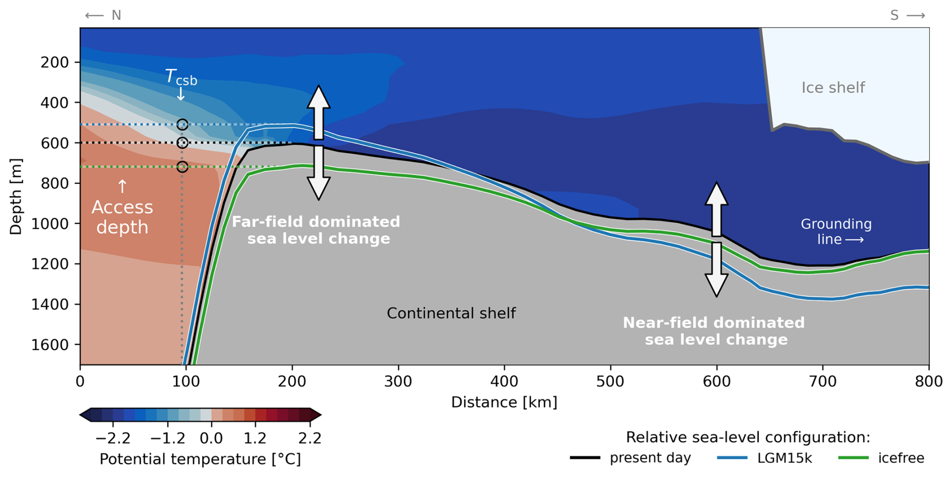
Figure 1 Schematic of a typical oceanic gateway, where topography shields a deep-lying grounding line from warm water inflow. A transect following the deepest topographic connection (along a trough) shows a common temperature distribution for the Antarctic continental shelf. Variations in the sill depth can occur in response to far-field and near-field variations in relative sea level, which affects the access depth from where offshore water masses flow onto the continental shelf. The effect of RSL changes on basal melt rates can be assessed by evaluating the change in ocean properties resulting from variations in access depths at the continental-shelf break (T_csb).

So far the effect of RSL changes on Antarctic basal melt rates has not been assessed. The importance and relevance of this effect are thus unclear as well as whether this mechanism should be considered for the ocean forcing in ice-sheet simulations. With this study we want to provide an approximate estimate on the potential impact of RSL change on basal melt rates in Antarctica. We first define different RSL configurations, which represent end-member realizations for past and future changes in sea level, as well as one RSL configuration related to an upper-end estimate of climatic change in the year 2300. From these RSL patterns we define a measure of open-ocean to grounding-line connectivity and compute its change for the Antarctic Ice Sheet. Subsequently, we infer how this changes the ocean properties that get access onto the continental shelf. By adding the derived changes in CSB temperature and salinities as anomalies to an ice-sheet model, we compute changes in basal melt rates based on the RSL signal.

The study consists of two different sets of experiments. In a first step, we test the sensitivity of a present-day ice-sheet configuration to end-member realizations of RSL change patterns to derive upper-limit estimates of this effect on basal melt rate changes. Secondly, we apply RSL-driven ocean-forcing corrections for specific past and future time slices of the Antarctic ice-sheet evolution to assess the effect of RSL-induced basal melt rate changes also in more realistic scenarios.

2 Methods

This section describes the methods and workflow we use to derive ice-shelf basal melt rate estimates by applying different RSL change configurations.

In order to assess the relevance and magnitude of relative sea level on basal melt rates, we define different configurations of RSL change. For an upper-limit estimate of past RSL changes, we choose the maximum ice extent of the AIS during the Last Glacial Maximum, which is named LGM15k in the following. For an upper limit of expected future changes, we assume a configuration where all present-day solid ice is melted and the global-mean sea level and solid Earth rebound would thus be highest (named icefree). For an intermediate and more realistic future setup, we also assess a configuration in the year 2300, with the Antarctic Ice Sheet being forced by an upper-limit climate projection (named yr2300). More information about these configurations is given below (Sect. 2.1.2).

To estimate sub-shelf melt rate changes for the different RSL configurations, we follow these steps:

1. Compute RSL changes with coupled ice-sheet–GIA simulations.

2. Identify access depths informed by RSL changes to determine open-ocean access to ice-sheet grounding lines.

3. Calculate ocean state changes at the continental-shelf break on the basis of vertical displacement of access depths.

4. Compute diagnostic changes in ice-shelf basal melt rates with an ice-sheet model.

In the following, we explain the methodology of each step in more detail.

2.1 Computation of RSL changes

In this section we first present the used models to compute RSL changes and then provide more information about the different RSL configurations that we use for our analysis.

2.1.1 Coupled ice-sheet–GIA model framework

We simulate RSL changes using the coupled ice-sheet–GIA model framework PISM-VILMA as described in Albrecht et al. (2024). The Parallel Ice Sheet Model (PISM; https://www.pism.io, last access: 29 January 2025; Bueler and Brown, 2009; Winkelmann et al., 2011), an open-source model which simulates ice sheets and ice shelves, is used to compute the transient evolution of the Antarctic Ice Sheet under external climatic forcing. It is interactively coupled to the VIscoelastic Lithosphere and MAntle model (VILMA; Klemann et al., 2008; Martinec et al., 2018), which calculates the solid Earth and sea-level response to changes in ice loading based on a 3D Earth structure (Bagge et al., 2021). VILMA solves the global sea-level equation self-consistently, which yields a sea-level fingerprint in response to the redistribution of water masses between ice sheets and ocean and is also a result of rotational and gravitational feedbacks. While Antarctic Ice Sheet changes are interactively modeled with PISM, ice evolution in the Northern Hemisphere is prescribed (see more information about this below in Sect. 2.1.2). PISM uses a regular Cartesian grid, with either 16 km (LGM15k) or 8 km (yr2300) horizontal resolution. VILMA utilizes a Gauss–Legendre grid, and our setup uses the n128 resolution (256 × 512 grid points) for viscoelastic deformation while solving the sea-level equation at higher resolution (n512, 1024 × 2048 grid points). We use the “3D ref” Earth rheology from Albrecht et al. (2024), which is equivalent to the “v_0.4_s16” configuration in Bagge et al. (2021). A visualization of the vertical and lateral viscosity structures in Antarctica as well as the lithosphere thickness is provided in Fig. 5 in Albrecht et al. (2024). VILMA is initialized with the global present-day ETOPO1 bed topography (Amante and Eakins, 2009; NOAA National Geophysical Data Center, 2009), where the Antarctic region has been replaced with the Bedmap2 dataset (Fretwell et al., 2013). Further information about the PISM-VILMA coupling framework is provided in Albrecht et al. (2024).

In order to represent the GIA response in the ice-sheet domain, we first calculate the change in relative sea level Δr(c) with respect to present-day RSL: r_pd=r(present-day), where r(c) denotes the new RSL of configuration c computed by PISM-VILMA (see Eq. 1). Subsequently, the present-day ice-sheet bedrock topography t_pd is corrected with the shift in RSL change to compute the updated bedrock t(c) (see Eq. 2).

$$\begin{array}{}\text{(1)}& {\displaystyle }\mathrm{\Delta }r\left(c\right)& {\displaystyle }=r\left(c\right)-r_{\mathrm{pd}}\text{(2)}& {\displaystyle }t\left(c\right)& {\displaystyle }=t_{\mathrm{pd}}-\mathrm{\Delta }r\left(c\right)\end{array}$$

We use the BedMachine Antarctica (v3) dataset (Morlighem, 2022; Morlighem et al., 2020) in original resolution (500 m) for present-day topography and regrid RSL changes Δr(c) from the VILMA to the BedMachine grid bilinearly.

2.1.2 RSL configurations

The LGM15k configuration represents the difference in relative sea level 15 kyr BP. It is extracted as a single time slice from a transient coupled ice-sheet–GIA simulation over the last 246 kyr BP (representing the last two glacial cycles) described in Albrecht et al. (2024). The Antarctic Ice Sheet is modeled with PISM, while the ice load history of the Northern Hemisphere is prescribed by the ICE-6G_C reconstruction (Stuhne and Peltier, 2015). The Antarctic climate forcing is scaled with temperature anomalies from ice-core reconstructions (Albrecht et al., 2020a). The coupled ice-sheet–GIA simulation of Albrecht et al. (2024) over two glacial cycles has been repeated six times to iteratively approach a suitable initial topography. This has been done by correcting the initial topography from 246 kyr BP with the offset between observational data and the modeled topography for the present day of the previous iteration, a typical procedure in paleo-GIA modeling to lower the present-day model–data misfit. The coupling interval between ice and GIA models is 100 years, and PISM uses a 16 km horizontal resolution. During the coupled simulation, the maximum AIS extent during the last glacial period is reached at around 15 kyr BP, which is approx. 11 000 years later than in the Northern Hemisphere (26 kyr BP; see Fig. S3). This delay agrees well with Clark et al. (2009), suggesting a West Antarctic LGM delay of 4.5–12 kyr with respect to the global LGM sea-level lowstand and the ICE-6G_C reconstruction. In our simulation, GMSL was approx. 93 m lower than today during that period.

The icefree RSL configuration is derived from the long-term solid Earth response to an instant removal of all present-day ice loads. Continental ice masses are redistributed as liquid water and added to the ocean mass, which leads to a GMSL rise of approx. 70 m in our simulation. As no dynamic ice-sheet changes are computed, this RSL configuration is computed with a VILMA standalone configuration. The simulation period spans 86 kyr into the future. The long simulation time has been chosen so that the full solid Earth response can unfold (before a possible next ice age), also in regions featuring high mantle viscosities as well as a thick lithosphere and therefore rather long response timescales.

The yr2300 RSL configuration is derived from a coupled PISM-VILMA simulation using an upper-limit climate forcing. The initial state for PISM is derived as in Reese et al. (2023), with a 400 kyr thermal spinup (using a 16 km horizontal resolution), followed by a 25 kyr full-physics spinup (8 km resolution). First, the historic period (1850–2015) is computed with pre-industrial climate forcing as described in Reese et al. (2023). The climate forcing for the subsequent model period (2015–2300) follows the ISMIP6 Antarctica 2300 protocol using an SSP5-8.5 realization of CESM2 (AE04; Seroussi et al., 2024). We use the best-scoring PISM ensemble member (AIS1) from Reese et al. (2023), which uses the following PISM parameters: till effective overburden fraction δ=1.75 % and till water content decay rate C_d=10 mm yr⁻¹. The coupling time step between PISM and VILMA is set to 1 year, and PISM uses an 8 km horizontal resolution. The historic period shows plausible RSL change rates (see Fig. S4) which are comparable to GNSS measurements (Willen et al., 2024; Buchta et al., 2024). While the climate forcing reflects an upper-end estimate, the dynamic ice-sheet response does not include structural uncertainties of ice-sheet behavior such as the marine ice cliff instability (MICI), which can potentially increase Antarctic ice loss by a factor of up to 4 but is poorly constrained (IPCC AR6 WG1 Chap. 9.6.3.5; Fox-Kemper et al., 2021). To also include non-Antarctic cryospheric changes and reflect redistributions in the global water budget, we add a uniform GMSL contribution of 3.68 m on the RSL changes computed by PISM-VILMA in a post-processing step (after the coupled simulation has been finished), which is composed from the upper end (83th percentile) of IPCC estimates for the year 2300 under SSP5‐8.5 forcing: the contributions are 1.75 m from the Greenland Ice Sheet, 0.32 m from glaciers, 0.10 m from land-water storage, and 1.51 m from thermal expansion (IPCC AR6 WG1 Chap. 9.6.3.5; Fox-Kemper et al., 2021, Table 9.11). By adding a uniform, global-mean sea-level offset to RSL changes computed by PISM-VILMA, we make the assumption that regional variations from the global mean around Antarctica, e.g., induced by gravitational or rotational effects in response to these contributions (with the origin mostly in the Northern Hemisphere), are small and not relevant on the scale of our assessment, which uses a vertical resolution of 1 m to identify access depths from topography.

2.2 Identification of access depths

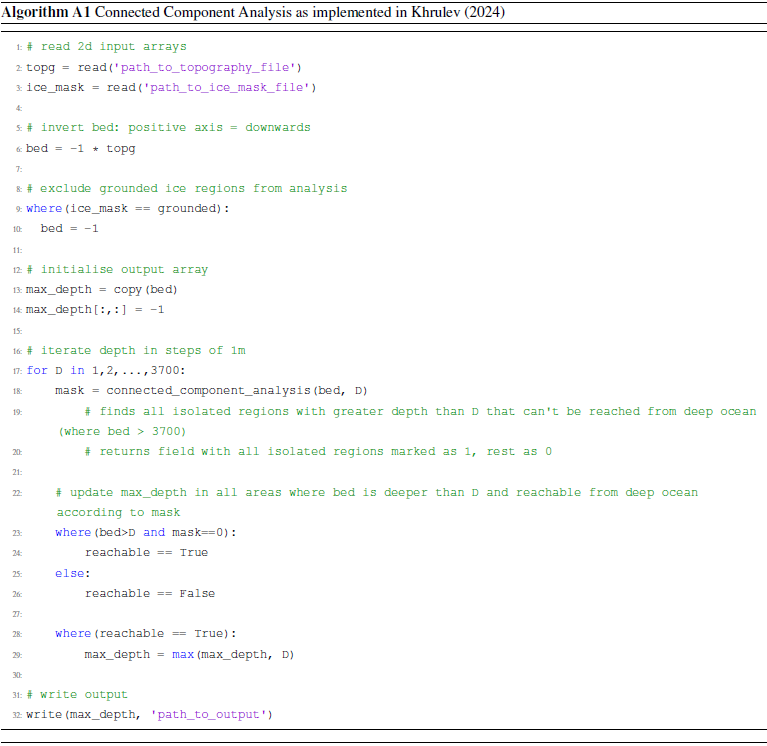
In order to evaluate how the altered bathymetry t(c) modifies the access of offshore water masses to the ice-sheet grounding lines, we make use of the approach developed in a related study by Nicola et al. (2025). Therein, oceanic gateways are defined as the deepest possible topographic connection of open-ocean water to the grounding lines of the Antarctic Ice Sheet. This methodology is based on the assumption that inflowing water masses from beyond the continental-shelf break always follows these deepest bathymetric pathways onto the continental shelf and eventually into the ice-shelf cavities. Overdeepened regions on the continental shelf are thereby shielded by shallower topography that inhibits the inflow of water masses from below the deepest connection to the open ocean. We systematically analyze the topographic connectedness by calculating an access depth map d_m(c). This map contains for every grid point on the continental shelf the largest possible depth for which there is a horizontal oceanic connection to the open ocean (which is defined as t>3700 m depth) that is not obstructed by bathymetry. We obtain the map of access depths d_m(c) via a “connected component analysis” (CCA) using the implementation by Khrulev (2025). The algorithm iterates the vertical water column from 0 to 3700 m depth at a vertical resolution of 1 m and finds isolated regions that can not be reached from locations classified as open ocean, as they are shielded by shallower topography. A pseudo-code version of the algorithm used is provided in Appendix A. Due to the efficient C++ implementation, an access depth map at 500 m resolution can be computed in less then 25 min using a single CPU core¹. We calculate access depth maps d_m(c) for each topography map t(c) including the present-day topography t_pd. Supplement Fig. S5 shows the access depth map d_m for the present day, and Fig. S6 shows the difference between bathymetry t(c) and the computed access depth maps d_m(c), which visualizes the location and magnitude by which deeper parts on the continental shelf are shielded by further offshore, more shallow topography. The influence of RSL changes Δr(c) on access depth maps can be analyzed through calculating the anomaly to present day:

$$\begin{array}{}\text{(3)}& \mathrm{\Delta }{d}_{\mathrm{m}}\left(c\right)=d_{\mathrm{m}}\left(c\right)-d_{\mathrm{m}}\left(\text{present-day}\right).\end{array}$$

From the inferred 2D access depth maps d_m(c), we select only the grid cells coinciding with the grounding-line mask for further analysis. The grounding-line mask is defined as all floating ice grid cells which have at least one of four possible direct neighboring cells with grounded ice belonging to the main Antarctic continent, which means that islands and ice rises are not considered here.

We evaluate the sparse access depth map at the grounding-line mask for different basins b and define the deepest access depth per basin as d_GL,0(b,c). Furthermore, we calculate access depths with the constraint that at least a certain fraction of the grounding line needs to be reached by this depth: d_GL,g(b,c) is the deepest possible access depth for RSL configuration c such that at least g % of the grounding-line cells in basin b have a deeper or similar access depth. Using a range of grounding-line fractions for $g\in \mathit{\{}\mathrm{10},\mathrm{20},\mathrm{\dots },\mathrm{90}\mathit{\}}$, we thereby obtain values of $d_{\text{GL,10}}(b,c),d_{\text{GL,20}}(b,c),\mathrm{\dots },d_{\text{GL,90}}(b,c)$ for each basin b and RSL configuration c. We use a classification of the AIS and the surrounding ocean from 19 basins as presented in Nicola et al. (2025), which are originally based on AIS drainage basins defined in Zwally et al. (2012), extended and modified by Reese et al. (2018) and adapted by Nicola et al. (2025) to match oceanic gateway pathways for the present day (basin boundaries shown in Fig. 2c). Changes in grounding-line access depths to the present-day baseline are computed as

$$\begin{array}{}\text{(4)}& {\displaystyle }\mathrm{\Delta }{d}_{\text{GL,0}}(b,c)=d_{\text{GL,0}}(b,c)-d_{\text{GL,0}}(b,\text{present-day}),\text{(5)}& {\displaystyle }\mathrm{\Delta }{d}_{\text{GL,g}}(b,c)=d_{\text{GL,g}}(b,c)-d_{\text{GL,g}}(b,\text{present-day}).\end{array}$$

Present-day topography features oceanic gateways, e.g., in the Filchner–Ronne basin (b=1) and the Amery basin (b=6) (Nicola et al., 2025). In the Filchner–Ronne basin around 80 % of the grounding line is reachable by water masses that overflow the topographic sill at d_GL,0=595 m. In the Amery basin this threshold is at 526 m depth, reaching ca. 65 % of the basin's grounding line. Oceanic gateways are also detected for example in the Ross basin (b=12) and the Amundsen Sea basin (b=14), where at the deepest open-ocean connection (570 and 575 m, respectively) 30 % of present-day grounding lines could directly be reached.

2.3 Calculation of marginal ocean properties

The underlying assumption of our methodology is that changes in the grounding-line access depth d_GL,0 modify the vertical entry point of water masses that flow onto the continental shelf from further offshore and thereby potentially affect the melting inside the ice-shelf cavities. We calculate this change in ocean properties by evaluating the vertical column of present-day ocean observations at the continental-shelf break for different access depths.

$$\begin{array}{}\text{(6)}& \begin{array}{rl}{T}_{\text{CSB, mean}}(b,c)& =\text{mean}\left\{\left.T(x,y,z)\right|(x,y)\in \text{CSB}\left(b\right)\right.\\ & \left.\text{ and }z=d_{\text{GL,0}}(b,c)\right\}\end{array}\end{array}$$

Hence T_CSB,mean is defined as the mean of ocean temperature T at the continental-shelf break at the depth of the deepest grounding-line access depth d_GL,0. We thereby define the CSB mask as all grid cells that are in the range of 40 km distance of the 1800 m isobath of present-day bathymetry. CSB(b) denotes the subset of the CSB mask in basin b. From the computed CSB temperatures for different RSL configurations c, we calculate the temperature anomaly with respect to the present-day configuration as

$$\begin{array}{}\text{(7)}& \begin{array}{rl}\mathrm{\Delta }{T}_{\text{CSB, mean}}(b,c)& =T_{\text{CSB, mean}}(b,c)\\ & -T_{\text{CSB, mean}}(b,\text{present-day})\end{array}\end{array}$$

and add them to baseline values used for calculating basal melt rates in ice-shelf cavities (see Sect. 2.4 and 2.5 below). Note that the anomaly method diverges from Nicola et al. (2025), who calculate ocean anomalies between the continental-shelf break and the calving front location in order to estimate the present-day basal melt increase due to extensive inflow of warmer offshore water masses into ice-shelf cavities.

Salinity values at the continental-shelf break S_CSB,mean and their anomalies to the present day ΔS_CSB,mean are computed according to Eqs. (6) and (7). Similar to Nicola et al. (2025), we make use of the ISMIP6 climatology dataset (Jourdain et al., 2020), which contains potential temperature and practical salinity data points averaged over the period 1995–2017 at an 8 km × 8 km horizontal and 60 m vertical resolution. The dataset is a combination of different data sources like the World Ocean Atlas 2018 (Locarnini et al., 2018; Zweng et al., 2019), the Met Office EN4 subsurface ocean profiles (Good et al., 2013), and the Marine Mammals Exploring the Oceans Pole to Pole (MEOP) dataset (Roquet et al., 2013, 2014; Treasure et al., 2017). Jourdain et al. (2020) merged and extrapolated these data products using a similar method to our CCA approach, which makes their data very suitable for our analysis, as missing data have been filled with appropriate values. To acquire ocean properties between discrete vertical data layers, we utilize linear interpolation along the vertical axis.

2.4 Computation of basal melt in ice-shelf cavities

For computing basal melt rates we use the Potsdam Ice shelf Cavity mOdule (PICO) as implemented in the ice-sheet model PISM (Reese et al., 2018). PICO parameterizes the vertical overturning circulation in ice-shelf cavities driven by melt-induced buoyancy fluxes, extending the box model by Olbers and Hellmer (2010) to two horizontal dimensions. The module takes ocean temperature and salinity from the floor of the continental-shelf area as input, typically averaged horizontally per basin, representing the water masses that reach the grounding line. Due to mixing with more buoyant meltwater, these water masses rise along the ice-shelf base via the ice-pump mechanism (Lewis and Perkin, 1986).

We compute basal melt rate changes in a pure diagnostic manner without any transient ice-sheet changes (except for one special case, explained in Sect. 2.5). Thus, the computed melt rates are solely dependent on the PICO parameters, the ocean forcing, and the ice-sheet geometry used. We compare “baseline” basal melt rates to ones that are obtained by adding RSL-derived ocean anomalies (ΔT_CSB,mean,ΔS_CSB,mean) to the baseline ocean forcing. Depending on the set of experiments, we use different ice-sheet geometries and resolutions (further information given below in Sect. 2.5).

PICO features two main (circum-Antarctic) parameters to adjust the amount of melting in the ice-shelf cavities: the vertical overturning circulation strength C (in Sv m³ kg⁻¹) and the heat-exchange coefficient ${\mathit{\gamma }}_T^{*}$ (in 10⁻⁵ m s⁻¹). Reese et al. (2023) tune these two parameters in order to represent realistic melt rate sensitivities for the given thermal forcing. Similar to the approach in Jourdain et al. (2020), they correct the input temperature values during this process, which are originally based on Schmidtko et al. (2014), in order to match present-day melt rate observations from Adusumilli et al. (2020). Which PICO parameters we use is explained in the following section.

2.5 Experiment design

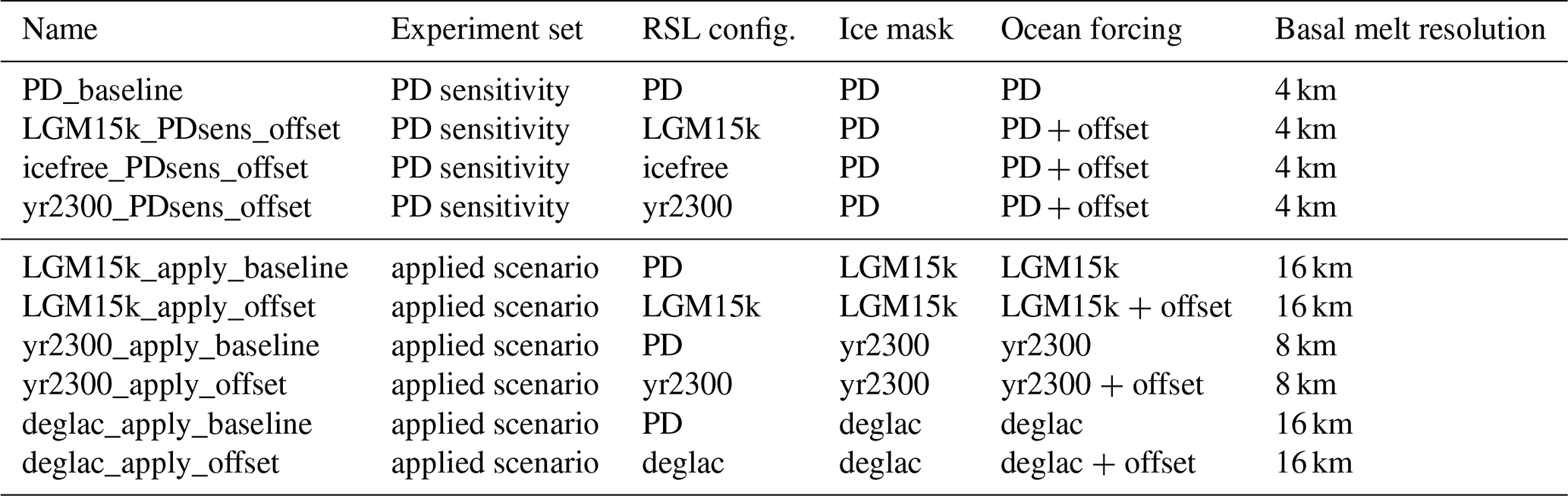
In order to estimate the impact of RSL changes on basal melt rates, we conduct different sets of experiments. They can be classified into the set of present-day sensitivity experiments and the applied scenario set, and they are all listed in Table 1.

Table 1 Experiment overview. A list of the experiments conducted for this study. RSL config. refers to the RSL configuration used to update the bedrock topography (c in Eqs. 1 and 2). Basal melt resolution indicates the horizontal resolution of the ice-sheet setup used for computing basal melt rates, and deglac represents a time series from LGM15k to the present day with 500-year time slices (more explanation in Sect. 2.5). PD stands for present day. Ocean-forcing offset refers to RSL-induced ocean anomalies ΔT_CSB,mean and ΔS_CSB,mean.

In the present-day sensitivity set we calculate the effect of different RSL configurations on basal melt rates using a present-day ice-sheet configuration. We thereby test for the sensitivity of present-day ice-shelf melt to RSL configurations from different (past and future) time slices which include the maximum range of plausible RSL changes. These experiments have no real-world application but are still useful in deriving upper-limit estimates of the maximum possible impact of relative sea level on basal melt rates.

The set encompasses the experiments LGM15k_PDsens_offset, icefree_PDsens_offset, and yr2300_PDsens_offset, where basal melt rates are compared to the present-day baseline experiment PD_baseline. We use an updated bedrock topography with the respective RSL configuration (see Eq. 2) to compute access depths d_GL,0(b,c) using the present-day ice-sheet mask and grounding-line position. Similarly, we compute access depths for PD_baseline, where no RSL changes are applied. We now add the derived changes in ocean forcing (ΔT_{CSB, mean},ΔS_{CSB, mean}; see Eq. 7) as an offset to the present-day baseline ocean forcing and compute basal melt rates with a present-day ice-sheet configuration. By comparing these melt rates to the baseline experiment, we acquire changes in ice-shelf basal melting driven by artificial RSL configurations for the present-day ice-sheet configuration.

To compute basal melt rates with PICO, we use bedrock topography and ice thickness from the BedMachine Antarctica (v3) dataset (Morlighem, 2022; Morlighem et al., 2020) regridded to a horizontal resolution of 4 km. We use the “best” parameter combination from Reese et al. (2023), which is {C= 2.0 Sv m³ kg⁻¹, ${\mathit{\gamma }}_T^{*}=\mathrm{5}\times {\mathrm{10}}^{-\mathrm{5}}$ m s⁻¹}. The baseline ocean forcing for this set of experiments corresponds to the temperature-corrected ocean input in Reese et al. (2023).

In the second, applied scenario set of experiments, we compute RSL-derived basal melt rate changes for ice-sheet configurations that correspond to the RSL configurations used. This experiment set is of a more realistic nature than the first one, as it considers the consistent ice-sheet geometry and corresponding ocean forcing that matches the RSL configurations used. It can therefore be regarded as an estimate of the RSL influence on basal melt rates in transient model simulations.

For the LGM15k and yr2300 RSL configurations, we first compute access depths and melt rates for a baseline scenario (*_apply_baseline) using the corresponding ice-sheet geometry and ocean forcing. Note that the bedrock topography is not updated in these baseline experiments, so no modifications to the ocean forcing due to RSL corrections apply. This is instead done in the subsequent experiments (*_apply_offset): the computed access depths d_GL,0 differ from the baseline experiments as the bedrock topography has been altered by the associated changes in RSL. Using Eqs. (6) and (7), we derive corrections in the ocean forcing. By comparing the computed basal melt rates from the *_apply_offset to the *_apply_baseline experiments, we compute the RSL impact on basal melt rates in real-world applications.

For the LGM15k scenario, the PICO parameters {C= 0.8 Sv m³ kg⁻¹, ${\mathit{\gamma }}_T^{*}=\mathrm{1}\times {\mathrm{10}}^{-\mathrm{5}}$m s⁻¹} are used at a horizontal grid resolution of 16 km, similar to Albrecht et al. (2020a). In the yr2300 case the “max” parameter set {C= 3.0 Sv m³ kg⁻¹, ${\mathit{\gamma }}_T^{*}=\mathrm{7}\times {\mathrm{10}}^{-\mathrm{5}}$m s⁻¹} from Reese et al. (2023) is used at a horizontal resolution of 8 km.

The applied scenario set features additional experiments named deglac_apply_baseline and deglac_apply_offset. These are similar to the LGM15k_apply_* experiments but encompass a time series for the whole deglaciation time span from 15 kyr BP to the present day in steps of 500 years. We compute the RSL-induced ocean-forcing corrections for every time slice using the same methodology as for the LGM15k case. We then repeat the coupled PISM-VILMA simulation for the deglaciation period and apply the ocean-forcing corrections as a time-dependent anomaly. The deglac_apply_offset experiment is the only one in this study for which we calculate basal melt rates with RSL-induced ocean corrections in a transient manner (compared to the pure diagnostic analysis for the other experiments).

3 Results

In this section we describe the results of our analysis investigating the impact of RSL change on Antarctic ice-shelf basal melt rates. First, we describe RSL changes for the LGM15k, icefree, and yr2300 configurations as modeled by the coupled ice-sheet–GIA simulations. The derived changes in grounding-line access depths are described thereafter before we assess the impact on CSB ocean temperatures, which drive the changes in basal melting. We present basal melt changes for the present-day sensitivity, as well as for the applied scenario experiment set.

3.1 Changes in relative sea level

Variations in the RSL pattern can be ascribed to barystatic, rotational, gravitational, or deformational processes. Hereafter, we will refer to changes in the far field, encompassing those arising from both barystatic effects and all GIA-induced alterations in the Northern Hemisphere that impact the Southern Hemisphere. This includes primarily the rotational component and alterations in ocean basin volume due to bedrock deformation linked to changes in ice load. In contrast, we categorize near-field effects as RSL changes resulting from GIA processes specific to the Antarctic Ice Sheet, primarily involving gravitational and deformational influences.

The LGM15k ice sheet features a well-advanced grounding line compared to the present-day location and a thicker ice column in almost all regions (see Fig. S7a). The increased ice thickness (up to +3000 m) is especially prominent in the marine basins, where today's largest ice shelves are located: the Filchner–Ronne (basin 1) and Ross basins (basin 12), as well as in large portions of the West Antarctic Ice Sheet (basins 13–16). To a lesser extent, thicker ice is also present in the Antarctic Peninsula (basins 17–19) and at the edges of East Antarctica. The interior of the East Antarctic Ice Sheet, however, shows a slight decrease in thickness during LGM15k (up to −140 m locally) due to less snowfall with colder surface temperature forcing (Nicola et al., 2023). The additional continental ice mass in Antarctica contributed around 15 m to the global-mean (barystatic) sea-level fall of 93 m at 15 kyr BP (130 m during the Northern Hemisphere LGM around 26 kyr BP).

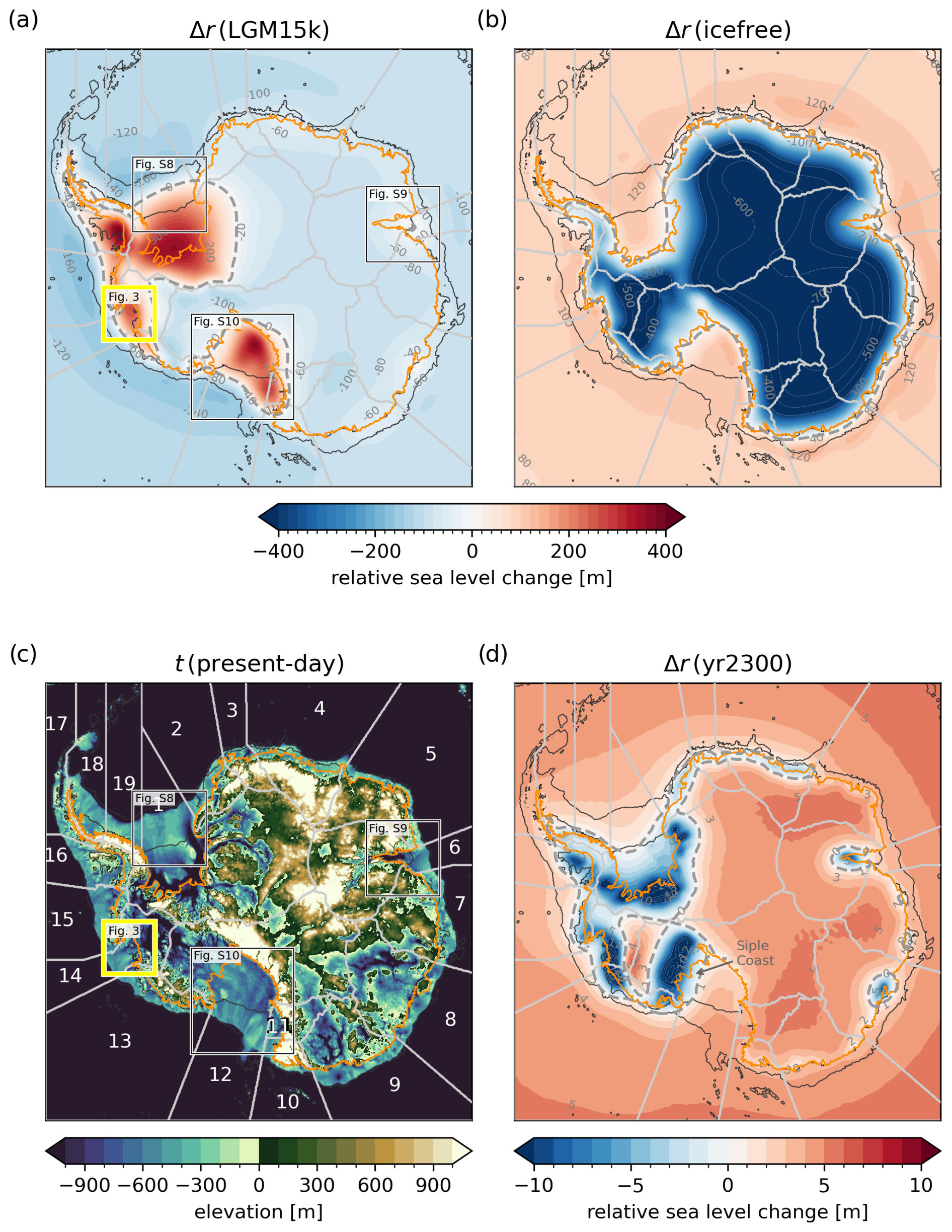
Figure 2 RSL changes for different configurations and present-day topography. Changes in relative sea level Δr are shown for LGM15k (a), icefree (b), and yr2300 (d) RSL configurations. The transition between positive and negative RSL changes is indicated by thick dashed gray contour lines. The grounding line of the present-day ice sheet is shown in orange, and the corresponding continental-shelf area (confined by CSB and present-day ice mask) is marked with black contour lines. Present-day reference topography t_pd (BedMachine v3) including basin numbers is shown in panel (c). The yellow rectangle indicates the Amundsen Sea basin, which is shown in more detail in Fig. 3. Close-up views of other regions are provided in Supplement Figs. S8 (Filchner–Ronne basin), S9 (Amery basin), and S10 (Ross basin).

The changes in sea level relative to the present day Δr as inferred from our coupled ice-sheet–GIA model are shown in Fig. 2 for different RSL configurations c. In the LGM15k case (Fig. 2a) the GIA response to greater ice extent overcompensates for the far-field sea-level fall in many parts: most of West Antarctica, the Filchner–Ronne and Ross basins, and parts of the Peninsula show a total RSL increase, which can be more than 400 m locally. This is also a consequence of the regionally weak Earth structure due to very low mantle viscosities and a thin lithosphere, which is represented in the 3D Earth structure used by VILMA (Bagge et al., 2021). In contrast, the LGM15k far-field sea-level fall dominates the RSL pattern in all regions of East Antarctica. Locally this RSL pattern is dampened through viscoelastic GIA effects, for instance in the Amery basin (b=6) or Totten basin (b=8), reflected by a reduction in the negative RSL signal in these regions (see Fig. 2a). The increased ice load leading to bedrock subsidence also causes a displacement of mantle material into the surrounding areas as part of the forebulge effect, which includes the elastic response of the lithosphere. This combined process further reduces the relative sea level in those areas and can be observed for example offshore of the Filchner–Ronne region ($b=\mathrm{1},\mathrm{19}$), in the Bellingshausen Sea (b=15), and in the Ross basin (b=12; see Fig. 2a).

In the icefree experiment, the transformation of all present-day ice masses into liquid water causes a barystatic sea-level rise of ca. +70 m. The VILMA output shows a strong bedrock uplift in all previously glaciated regions in both hemispheres (see Fig. 2b). The solid Earth response causes uplift (RSL decrease) of up to 800 m in the interior of the AIS. The mantle material is drained from the surroundings, causing an inverse forebulge effect, such that the RSL increases approx. 20 m more than the far-field sea-level rise in many places of the present-day continental-shelf area. Areas where the far-field increase in sea level and the near-field bedrock uplift compensate for each other (dashed gray contour line in Fig. 2b) are found close to present-day grounding lines.

The simulated ice sheet in the yr2300 case shows significant grounding-line retreat from the present-day location, especially in the Filchner–Ronne region (b=1); the Siple Coast, which is part of the Ross Ice Shelf (b=12); parts of the Antarctic Peninsula ($b=\mathrm{16},\mathrm{18},\mathrm{19}$); and the West Antarctic basins (b=13–15). Also in Dronning Maud Land (b=2–4), the Amery basin (b=6), and the Totten region (b=8), widespread grounding-line retreat can be observed (see Fig. S7b). The far-field signal in RSL change is mostly in the range of 4–5 m in the Southern Ocean (see Fig. 2d). Bedrock uplift caused by grounding-line retreat and ice-sheet thinning reduces the depth of the water column in locally strongly differing magnitudes. In regions of strong uplift, like for instance in the West Antarctic basins, the Antarctic Peninsula, the Filchner–Ronne basin, and the Siple Coast, relative sea level shows a net decrease (up to −19 m), overcompensating for the far-field sea-level rise. The far-field signal is dominant in large parts of East Antarctica with some exceptions, like in Dronning Maud Land, the Amery basin, or the Totten region.

3.2 Changes in access depths

We compute the updated topography t(c) for each RSL configuration c (Eq. 2) using the changes in relative sea level Δr presented above. Based on this, we compute access depth maps d_m(c) and retrieve the grounding-line access depths d_GL,0(b,c) and d_GL,g(b,c) as explained in Sect. 2.2. In this section, we explain the relation between d_m and d_GL,g exemplary for the present-day sensitivity experiment set. The applied scenario experiments use the same RSL changes Δr(c) but feature different ice masks and thereby grounding-line positions. Results from this set are shown further below (Sect. 3.4). Results for d_GL,0 are shown in Sect. 3.3 and 3.4.

In order to understand how changes in relative sea level (Δr) translate to differences in access depth maps (Δd_m) and subsequently to changes in grounding-line access depths (Δd_GL,0 and Δd_GL,g), it is helpful to examine the spatial patterns in detail. Figure 3 shows the present-day bedrock topography t_pd, the RSL change Δr, the present-day access depth map d_m(present-day), and its associated change (Δd_m) for the LGM15k RSL configuration in the Amundsen Sea Embayment (basin 14).

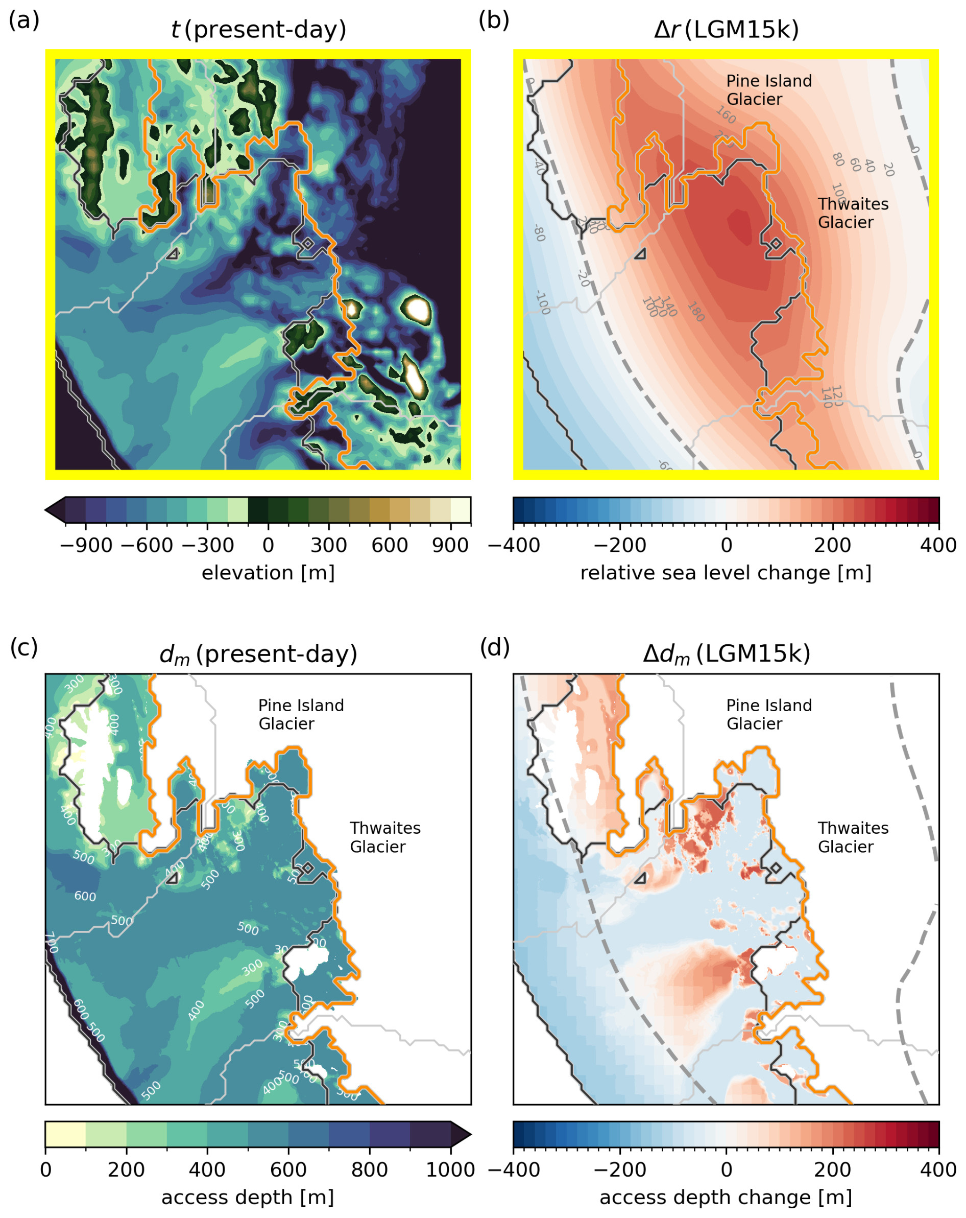
Figure 3 Influence of RSL change on access depths in the Amundsen Sea Embayment for the LGM15k RSL configuration. The upper row shows present-day topography t_pd (a) and the change in relative sea level Δr in the LGM15k configuration (b), which are both close-up views of Fig. 2. Lower panels show the derived access depth map d_m for present-day bathymetry (c) and the corresponding change Δd_m for LGM15k (d). The present-day grounding line is shown in orange, and the continental-shelf area (excluding floating ice) is marked with black contour lines. The zero contour line of RSL changes is marked as a dashed gray line in panels (b) and (d). Yellow borders refer to map extent highlighted in Fig. 2. The Amundsen Sea Embayment region shown here is labeled as basin 14 in our analysis, with adjacent basins 15 (above) and 13 (below) separated by thin gray lines.

There, a relatively shallow sill at the front of the continental shelf (see Fig. 3a and c) hinders water masses to reach deeper regions further inland including the present-day grounding line. RSL change at the outer regions of the continental shelf is dominated by the far-field sea-level fall, which reduces the sill depth (meaning the sill is getting shallower; see Fig. 3b). In contrast, relative sea level increases by several hundred meters in the interior of the ice-shelf basin due to increased ice loading and subsidence of the bedrock, overcompensating for the far-field sea-level fall. These two opposed signals of RSL change are also represented in the introductory schematic (cyan line in Fig. 1). Despite the clear pattern of RSL changes in the Amundsen Sea region (Fig. 3b), the horizontal fingerprint of access depth changes is very heterogeneous (Fig. 3d): it is generally dominated by the sea-level fall at the sill, meaning that bedrock subsidence has no additional effect in the over-deepened interior. A deepening of the access depth only occurs in regions where present-day topography is higher than the overflow sill (compare Fig. 3a, c and d).

To derive grounding-line access depths d_GL,g, we evaluate the spatial access depth map d_m at the position of the grounding line. Figure 4 shows grounding-line access depths d_GL,g for different RSL configurations in the present-day sensitivity experiments and their differences from present-day depth (Δd_GL,g; panel b). Using a present-day ice-sheet geometry and the RSL configuration LGM15k, the deepest 40 % of the grounding line in the Amundsen Sea basin is accessible by shallower ocean water compared to the present (up to 78 m) as a result of the far-field decrease in sea level (see Fig. 4b, basin 14). Note that the grounding line in the Amundsen Sea has many small patches with higher elevation than the sill at the outer continental shelf, which are not clearly recognizable in Fig. 3d. Shallower parts of the grounding line are instead reached by deeper waters compared to the reference (up to 204 m), as these regions are subject to bedrock subsidence (see Figs. 3b and 4d). This enhances the “oceanic gateway feature” drastically in the sense that a larger share of the grounding line could be reached at the deepest possible access depth: in the LGM15k case, 75 % of the grounding line is in reach via the deepest grounding-line access depth (497 m), whereas the deepest connection for the present day covers only 30 % (575 m; compare blue and orange bars in Fig. 4a, basin 14).

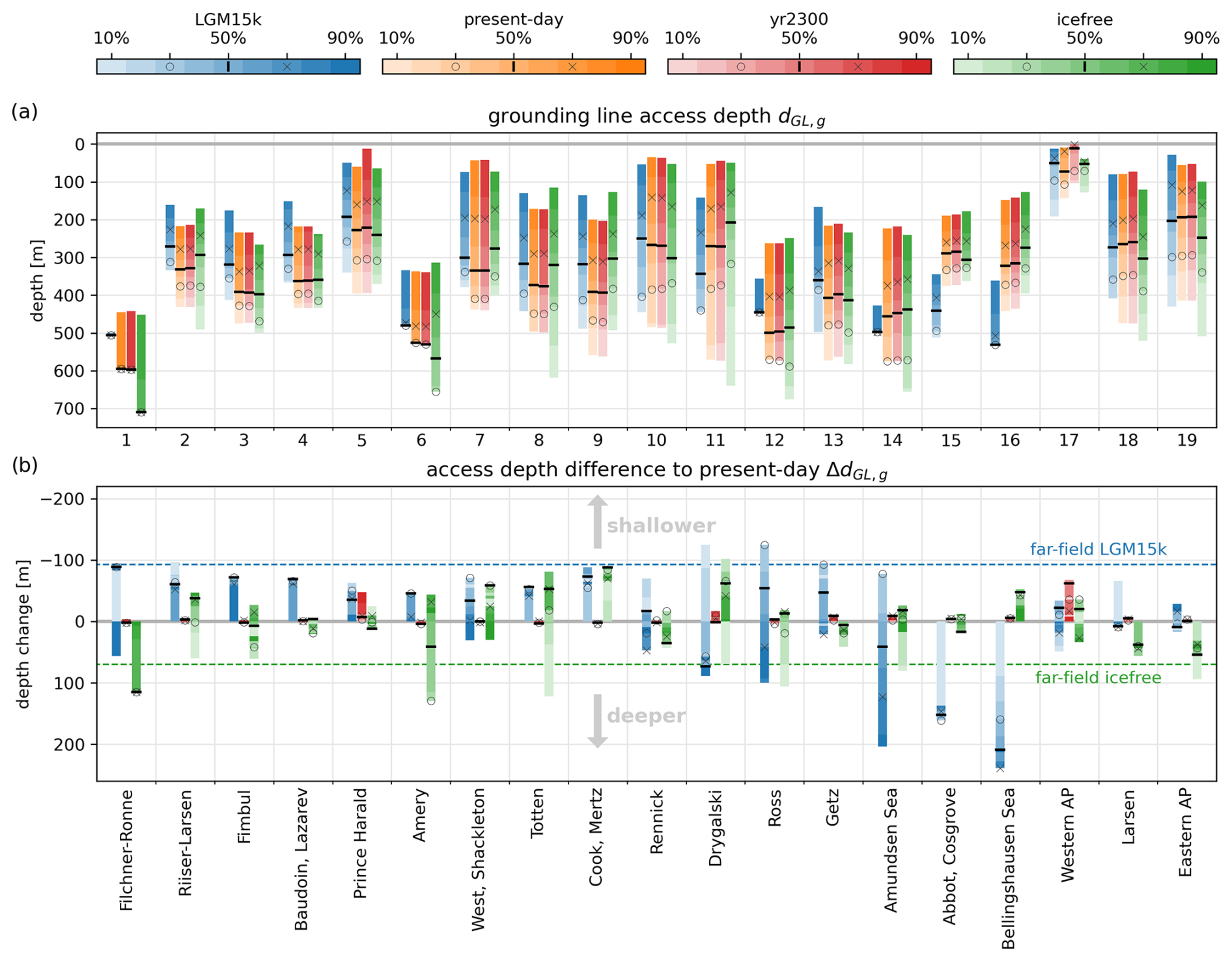
Figure 4 Grounding-line access depths d_GL,g (a) and their changes compared to the present day Δd_GL,g (b). The color shade indicates the percentage of grounding line reached by the specific access depth, with additional marks for d_GL,30 (o), d_GL,50 (–), and d_GL,70 (x). Barystatic sea-level changes are indicated by dashed horizontal lines in panel (b) for LGM15k and icefree RSL configurations. The plot shows results for the present-day sensitivity experiment set, which uses a present-day ice mask and grounding-line position but updated topography. Basins are labeled according to prominent ice shelves following Nicola et al. (2025). AP signifies Antarctic Peninsula.

In the LGM15k configuration, barystatic sea level is about 93 m lower than today, which at first estimate would make grounding-line access depths uniformly shallower in all basins when only the far-field sea-level change with some distance to the AIS was considered. This is indicated by a dashed horizontal line in Fig. 4b. As seen in the Amundsen Sea Embayment, deviations from this line are caused by the combination of different factors like the horizontal fingerprint of RSL changes, the bedrock topography (retro- or prograde slope), and the position and depth of the grounding lines.

Furthermore, the sign and strength of Δd_GL,g depends on the fraction of grounding line g that is considered. Also in other basins we observe a mixed signal in grounding-line access depth change for the LGM15k RSL configuration, namely in basins 1, 7, and 10–13, with the deepest grounding-line access depths getting shallower, while the higher grounding-line parts are getting deeper. In most of the East Antarctic basins (b=2–6, 8, 9) Δd_GL,g gets shallower for all values of g. The maximum reduction in grounding-line access depth is, however, less than the far-field sea-level fall, when bedrock subsidence dampens the RSL signal locally. In West Antarctic basins 15 and 16, the whole grounding line shows deeper access depths compared to the present day, as the bedrock subsidence overcompensates for the far-field sea-level fall and no prominent oceanic gateway features exist during the present day in these basins (Nicola et al., 2025). The presence of even shallower grounding-line access depths compared to the far-field sea-level fall in basin 12 is explained by the forebulge effect in the respective continental-shelf region (see Fig. 2a). Similar plots to Fig. 3 are added in the Supplement, namely for the Filchner–Ronne basin (b=1; Fig. S8), the Amery basin (b=6; Fig. S9), and the Ross basin (b=12; Fig. S10).

Figure 4 shows grounding-line access depths and their changes also for the icefree and yr2300 RSL configurations of the present-day sensitivity experiment set. In the icefree case Δd_GL,g is in the range of −102 to +129 m and thereby of the same order as the far-field barystatic sea-level rise of +70 m. The maximum deepening of grounding-line access depths partly exceeds the far-field signal (basins 1, 6, 8, and 12) due to a reverse-forebulge effect, where uplift in the interior of the Antarctic continent leads to the draining of mantle material in the vicinity, which causes an increase in the RSL rise.

As stated above in Sect. 3.1, Δr is between +5 and −19 m for the yr2300 RSL configuration, which is an order of magnitude smaller than the other cases. Due to the scale, most of the changes to the present day are therefore not clearly recognizable in Fig. 4b, with two exceptions: Δd_GL,g is up to −72 m in basin 17 and up to −54 m in basin 5. Deviations greater than 20 m are found only for high grounding-line fractions (g≥70 %) in the latter case. The validity of basin 17 results is generally questionable, as this basin features only very little grounding-line grid cells for the present-day ice-sheet configuration. Note that grounding-line access depths in basin 17 are much shallower compared to the other basins (Fig. 4a), which leads to a high gradient of grounding coverage g to d_GL,g. Subsequently, small values in Δr can lead to comparably high Δd_GL,g.

3.3 Present-day sensitivity experiments

The presented changes in relative sea level (Sect. 3.1) and access depth (Sect. 3.2) give a general understanding of how GIA processes influence the connectivity of open-ocean water to ice-sheet grounding lines. In this section, we carry out the next step of our analysis and analyze how the changes in grounding-line access depth influence the water properties (ocean temperature and salinity) that potentially reach the grounding lines, as well as what changes in basal melting thereby occur. Water properties on the continental shelf, extrapolated up to the grounding line, are generally used as input to PICO, which mimics the ice-pump mechanism, assuming that (melt) water rises upwards from the grounding line along the ice-shelf draft (see Sect. 2.4). In the following, we thus consider only the deepest grounding-line access depth d_GL,0 and its changes. Note that this section is about the sensitivity of basal melting for present-day ice-shelf geometries to different RSL configurations (upper section of Table 1), while results for different ice-sheet geometries are presented in the following (Sect. 3.4).

Figure 5 shows the changes in deepest grounding-line access depth Δd_GL,0, the derived modifications in mean temperatures along the continental-shelf break ΔT_csb,mean, and the resulting changes in basal melt rates for the set of present-day sensitivity experiments (LGM15k_PDsens_offset, icefree_PDsens_offset, and yr2300_PDsens_offset). The experiments are compared to the present-day baseline experiment PD_baseline (see Sect. 2.5 for details). Note that results for basin 11 are not shown as there is no continental-shelf region associated with this basin. Absolute basal melt rates are shown in Fig. S11 (PD_baseline) and Fig. S12 (*_PDsens_offset).

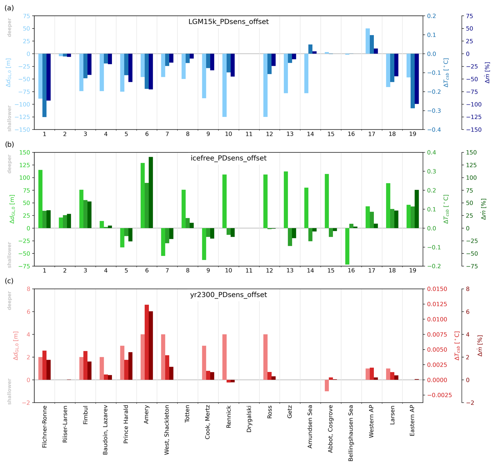
Figure 5 Changes for grounding-line access depth, ocean temperatures, and basal melt rates (present-day sensitivity experiments). The plot shows for each basin (from left to right) change in grounding-line access depth (Δd_GL,0), change in CSB temperature (ΔT_csb,mean), and relative change in basal melt rates ($\mathrm{\Delta }\dot{m}$) compared to baseline experiment PD_baseline. Bar colors correspond to the respective y axis. Note that the y-axis orientation for Δd_GL,0 is reversed compared to Fig. 4 to be aligned with the orientation of ΔT_csb and $\mathrm{\Delta }\dot{m}$.

For LGM15k_PDsens_offset, access depth changes Δd_GL,0 are up to 125 m shallower due to the applied RSL change (Fig. 5a). Only basins 15 (+3 m) and 17 (+50 m) have deeper access depths. The shallower grounding-line access leads to negative CSB temperature anomalies at different magnitudes (−0.02 °C in basin 2 to −0.33 °C in basin 1), which is due to the varying thermocline gradients per basin (see Fig. S1). Basin 14 is the only region with a sign reversal between access depth change (−78 m) and temperature anomaly (+0.05 °C), as the present-day access depth (575 m) is below the thermocline layer, so temperatures increase when moving up the water column from there (see Fig. S1). The negative temperature anomalies lead to a reduction in basal melting, which is up to −100 % (basin 19) compared to present-day melt rates. Relevant positive changes in basal melt rates occur only in basin 14 (+5 %) and basin 17 (+10 %).

The sensitivity of the icefree RSL configuration to the present-day ice sheet (icefree_PDsens_offset; Fig. 5b) is more heterogeneous across the basins, as indicated in previous results (see Δd_GL,g in Sect. 3.2). Access depth changes range from +129 m (deeper) in basin 6 to −72 m (shallower) in basin 16. The relationship between access depth change and temperature anomaly follows the same direction for all basins except 10–16, where it is inversed, as the present-day grounding-line access depths are at the thermocline maximum or below in these basins (see Fig. S1). The maximum derived temperature change at the continental-shelf break due to the RSL corrections ranges from +0.24 °C (basin 6) to −0.09 °C (basin 13). The derived basal melt rate changes range from more than doubling (+141 %) in basin 6 % to −26 % in basin 5.

Applying the yr2300 RSL configuration to the present-day ice sheet (yr2300_PDsens_offset; Fig. 5c) results in mostly deeper access depths (up to 4 m) and temperature anomalies between −0.001 °C (basin 10) and +0.012 °C (basin 6), which would change present-day melt rates by up to 6 % at maximum.

3.4 Applied scenario experiments

Testing the sensitivity of a present-day ice-sheet with end-member RSL configurations is useful for an upper-bound estimate of the RSL change impact on basal melting, but changes possibly deviate for different ice-sheet configurations. This section shows the results for RSL-induced basal melt rate changes using the respective ice-sheet configuration from where the RSL configurations LGM15k and yr2300 have been derived. The icefree RSL configuration is not included as in this scenario there is no ice sheet to compute basal melt rate changes for.

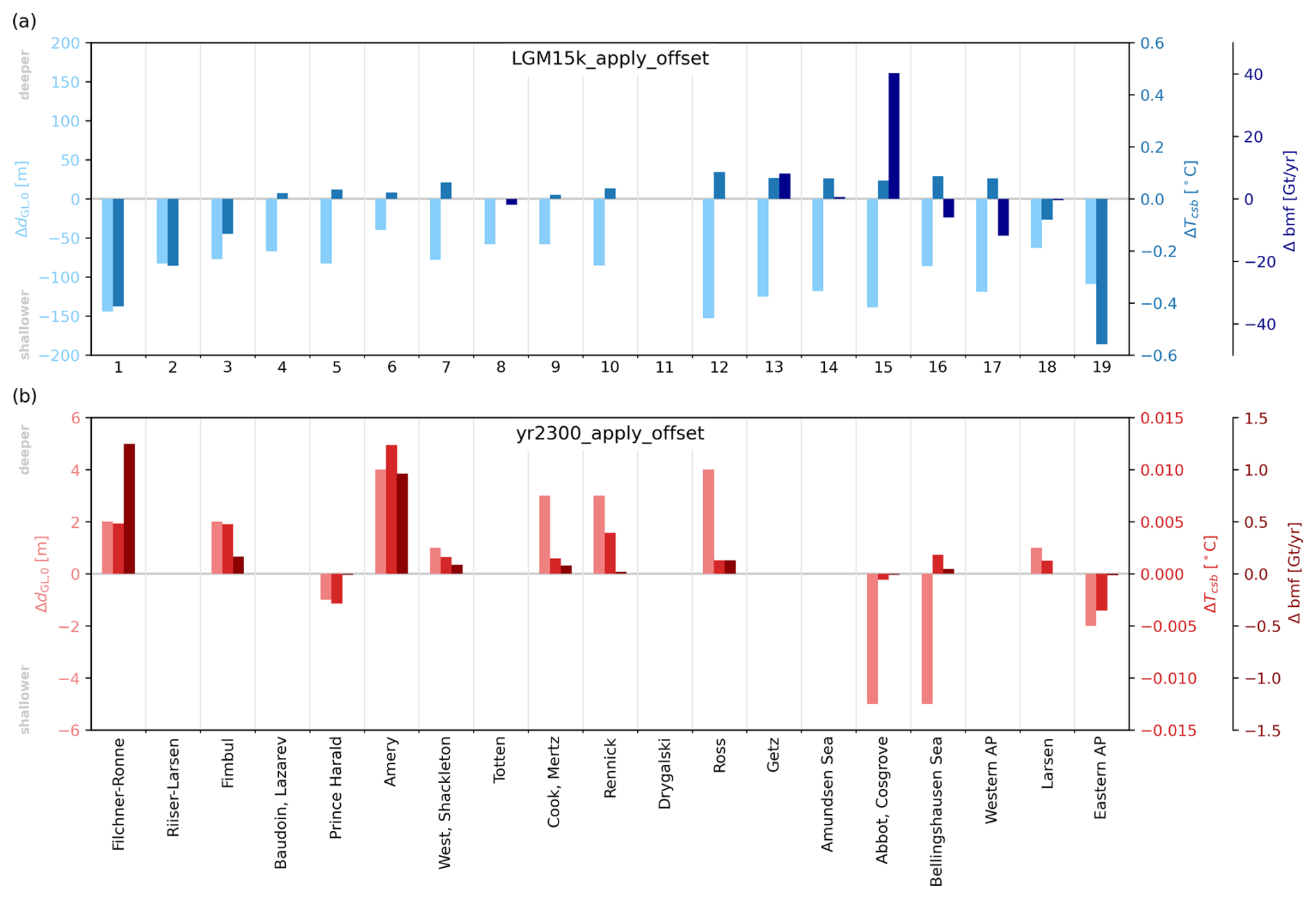
Figure 6 Changes for grounding-line access depth, ocean temperatures, and basal melt rates (applied scenario experiments). Similar to Fig. 5, but anomalies are computed to LGM15k_apply_baseline and yr2300_apply_baseline experiments. Other than in Fig. 5, changes in basal melting are displayed as absolute basal mass flux differences, which is more adequate as basal melting is close to zero in many basins of LGM15k_apply_baseline.

Grounding-line access depths d_GL,0 are 40–153 m shallower in the LGM15k_apply_offset experiment compared to LGM15k_apply_baseline (Fig. 6a), resulting in CSB temperature changes between −0.55 and +0.10 °C. Note that Supplement Figs. S1 and S2 show the dependence of temperature and salinity values on their respective grounding-line access depths for the baseline and “offset” experiment. The ocean-forcing temperatures in LGM15k_apply_baseline are generally cold enough to suppress any relevant basal melting during the LGM except in the West Antarctic basins including the western Antarctic Peninsula (basins 13–17; see Fig. S11b), as melt computed by PICO is confined by the pressure melting point. Therefore, these are the only basins where a change in basal mass flux can be observed when applying the RSL-derived temperature correction ΔT_csb,mean to the baseline forcing. The resulting basal mass flux changes range from −12 to +40 Gt yr⁻¹, which relates to relative changes of −15 % (basin 17) and +41 % (basin 15) compared to the baseline.

In order to test whether the RSL correction changes the transient evolution of the Antarctic Ice Sheet during deglaciation, we calculate in the deglac_apply_offset experiment the temperature correction T_csb,mean of LGM15k_apply_offset for every 500 years since 15 kyr BP and apply it as a temperature correction to the transient ice-sheet forcing in the coupled PISM-VILMA simulation. Figure 7 shows the transient sea-level-equivalent AIS volume with and without our temperature correction applied. After ca. 2 kyr of the coupled deglaciation simulation with applied RSL temperature correction, the ice loss since the LGM is slightly delayed compared to the baseline run (deglac_apply_baseline). Within the last 5 kyr of the run, ice loss is slightly faster with the RSL correction applied. The difference in ice volume above floatation for the present day is around 0.4 $\mathrm{m}\mathrm{s}.\mathrm{l}.\mathrm{e}.$, which is relatively small compared to the modeled difference of 14 $\mathrm{m}\mathrm{s}.\mathrm{l}.\mathrm{e}.$ between the LGM and present day and the difference of different VILMA rheology parameters (see Fig. 7b in Albrecht et al., 2024). The RSL correction implies both positive as well as negative temperature anomalies, depending on the basin and model time. Access depths and corresponding continental-shelf temperatures as well as PICO input temperatures are shown for different basins and the deglaciation time span in Fig. S13. In general, the applied RSL correction is substantially smaller than the climate-induced variation in PICO forcing over time, which explains the comparably small effect of RSL change on melting and the AIS evolution throughout the deglaciation simulation.

The applied yr2300 experiment (yr2300_apply_offset) provides comparable results to yr2300_PDsens_offset: changes in grounding-line access depths are in the range of ±5 m, which results in a comparable change in CSB temperature anomalies ($\le \pm \mathrm{0.012}$ °C). Absolute changes in basal mass flux that result from this RSL adjustment are less than 1.5 Gt yr⁻¹. Compared to yr2300_PDsens_baseline, these changes are less than 0.4 %, which is smaller than those in the present-day sensitivity experiment, as climate forcing and basal melting in the 2300 projection are substantially higher (see Fig. S11a and c).

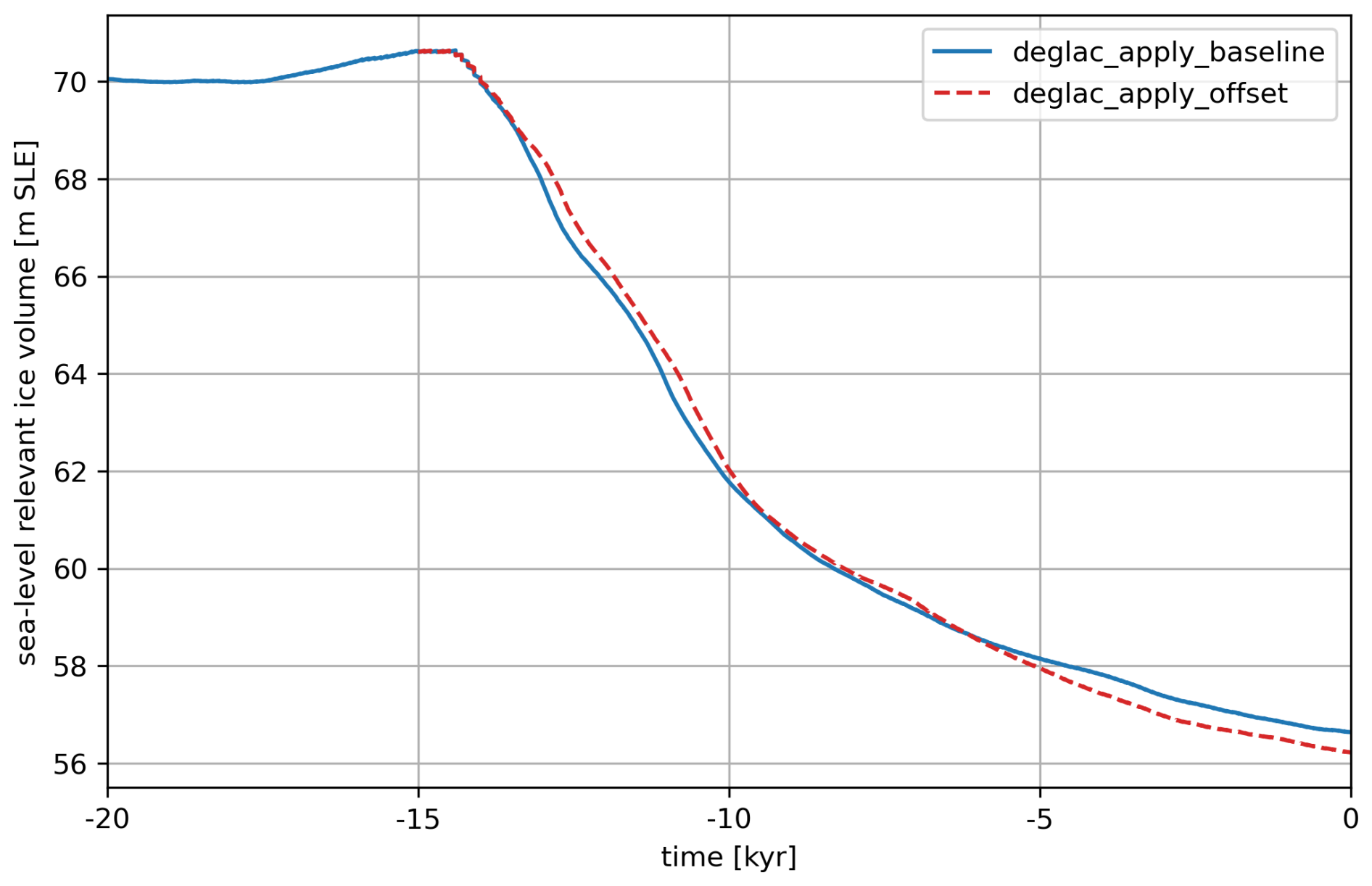
Figure 7 Influence of RSL correction on the deglaciation of the Antarctic Ice Sheet (in m s.l.e.).

4 Discussion

In this section we will critically review the methods we used to derive our results, discuss possible limitations, and give context to the results. Some important points have already been addressed in Nicola et al. (2025), as for instance the dependence of the results on the sub-shelf melt parameterization (Burgard et al., 2022), the chosen melt parameters for the PICO model or the influence of basin boundaries.

So far, we have derived our results using a single set of PICO parameters for the present-day sensitivity experiment set {C= 2.0 Sv m³ kg⁻¹, ${\mathit{\gamma }}_T^{*}=\mathrm{5}\times {\mathrm{10}}^{-\mathrm{5}}$m s⁻¹}, which is tuned to represent present-day melt rate sensitivities best (see Sect. 2.5 and Reese et al., 2023). In order to test the influence of PICO parameters on our results, we repeat the analysis with an additional set of PICO parameters, representing the maximum sensitivity to present-day melt rate changes, which is {C= 3.0 Sv m³ kg${}^{-\mathrm{1}},{\mathit{\gamma }}_T^{*}=\mathrm{7}\times {\mathrm{10}}^{-\mathrm{5}}$m s⁻¹} (cf. Reese et al., 2023). Additionally, we test the robustness of our results by deriving the ocean anomalies (ΔT_csb,mean,ΔS_csb,mean; Eqs. 6 and 7) not only as the mean along the continental-shelf break, but also as maximum values (ΔT_csb,max,ΔS_csb,max). The influence of PICO parameters in the PD_baseline experiment is comparably small in all regions with exceptions in basins 15–17 (see Fig. S12). Accordingly, the influence of the temperature selection method (mean vs. maximum along the continental-shelf break) is larger than the influence of the chosen PICO parameters, in all basins except 15–17 (see Fig. S12).

Note that we have focused on temperature changes at the continental-shelf break throughout this paper, as they are far more important for the melting response than salinity anomalies: according to the melt rate estimate depending on the equation of state (Eq. 8; Reese et al., 2018), a temperature anomaly of 0.5 °C has a 40 times larger effect on melt than a change of 0.2 psu in salinity ($\mathrm{0.5}\mathrm{°}\mathrm{C}/(\mathrm{0.0572}\mathrm{°}\mathrm{C}{\mathrm{psu}}^{-\mathrm{1}}\cdot \mathrm{0.2}\mathrm{psu})\approx \mathrm{43.7}$).

The RSL configurations used in this study were informed by coupled PISM-VILMA simulations, which account for the 3D structure of the solid Earth, including laterally varying lithosphere thickness and mantle viscosity. Again, we have used only a single 3D Earth rheology configuration (named “3D ref” in Albrecht et al., 2024, and “v_0.4_s16” in Bagge et al., 2021) for our analysis, which shows the best fit to global RSL records (Bagge et al., 2021) and represents spatially varying parameters between West and East Antarctica (see Fig. 5; Albrecht et al., 2024). However, there is still considerable uncertainty in the parameter space (van Calcar et al., 2023), which has the potential to change the response in grounding-line access depth. Albrecht et al. (2024), for example, show that a thinner lithosphere and low mantle viscosities, as likely dominant in West Antarctica, support a larger ice-sheet extent (sea-level-equivalent Antarctic ice volume can be a few meters larger) and much stronger bedrock subsidence (of the order of hundreds of meters) when considering large and long-term changes in climate forcing. By comparing three additional rheology configurations (“3D ant”, “3D trans”, and “3D glob”; see supplementary material of Albrecht et al., 2024), we see diverging RSL changes of up to 200 m during the LGM, especially in the Filchner–Ronne basin. It cannot be completely ruled out that the VILMA parameters have a non-negligible effect on our results. However, the 3D ref rheology we used for our results already represents the upper end of tested RSL changes. As systematic testing of the different VILMA parameter sets is beyond the scope of this study, this remains future work.

The applied scenario experiments rely on ice-sheet simulations with prescribed climate forcing. The corresponding LGM15k and deglaciation experiments make use of a climate-index method to scale external forcing temperatures (ocean and atmosphere) by ice-core reconstructions (Albrecht et al., 2020a). In the yr2300 experiment, climate anomalies from the global climate model CESM2 are used according to the ISMIP6 Antarctica 2300 protocol (Seroussi et al., 2024). We compute CSB ocean anomalies based on the present-day ISMIP6 dataset by Jourdain et al. (2020) for all experiments and add these to the respective baseline forcing despite the discrepancy between it and present-day climate conditions. The underlying assumption that any climatic changes in the ocean are uniform with depth is often inaccurate and warrants further scrutiny.

Our approach of applying CSB ocean anomalies derived from access depth changes directly to the oceanic input at the grounding lines has a number of further limitations. First of all, we fully rely on the ISMIP6 dataset to represent the current ocean state at the continental-shelf break realistically. Despite the fact that this dataset merges different available data sources (argo floats, ship cruises, satellites, and marine mammals), in situ observations at the Antarctic continent margin still remain sparse in temporal and spatial resolution. Furthermore, our approach does solely rely on the vertical ocean profile and does not reflect other mechanisms: for example, if the grounding-line access depth is below the thermocline layer, a change in access depth has little effect on the derived ocean anomaly. However, a thicker layer of intruding CDW, which is likely with RSL increase, has the potential to modify basal melting substantially.

A general downside of the anomaly approach is that we do not account for any changes in cross-shelf water transport including the modification of water masses on the continental shelf. The processes that regulate the transport of warm offshore waters onto the continental shelf and towards grounding lines are inherently complex and governed by many factors: e.g., topographic features, strength and location of sea-ice formation, wind patterns, precipitation, ambient air temperature, freshwater input through basal melting, or tides; see Thompson et al. (2018) and Colleoni et al. (2018) for detailed reviews. Moreover, as mentioned in the Introduction, there is evidence that GIA processes themselves control ocean circulation on the continental shelf and offshore (Rugenstein et al., 2014; Wilmes et al., 2017; Tinto et al., 2019), which is not covered by our methodology. According to Thompson et al. (2018), the Antarctic continental shelf can be classified into three distinct types, namely fresh, dense, and warm shelf regions, which differ in terms of ocean dynamics and water mass exchange across the continental-shelf break. Fresh shelves are characterized by a strong Antarctic Slope Current with little cross-shelf water mass exchange. Dense shelves feature moderate exchange with efficient pathways for both import of CDW and export of Dense Shelf Water. Warm shelves typically exhibit a weak frontal structure which allows for high water mass exchange across the continental-shelf break and almost uninhibited access of CDW to the continental shelf (Thompson et al., 2018). Our anomaly approach is best suited for warm shelf regions, as there is a direct relationship between the CSB temperatures and the water masses on the continental shelf that enter the ice-shelf cavities. Despite the methodology being less suited for dense and fresh continental-shelf regions, it is still valuable for deriving upper-bound estimates of basal melt changes, as the actual changes represent an attenuation.

High-resolution ocean modeling can help us to study the dependence of ocean processes on RSL changes that are not captured by our methodology: a change in isopycnal slopes at the continental-shelf break, changes in thermocline gradients, transport of open-ocean water masses onto the continental shelf, or how ocean circulation inside the ice-shelf cavities is affected. This possibly requires cavity-resolving ocean model domains down to kilometer-scale resolution. Additionally, representing different time periods with significantly varied climate conditions and ice-sheet configurations is also required, e.g., the Last Glacial Maximum or climate projections for the year 2300. Considering the long simulation run times and extensive computational costs associated with high-resolution ocean modeling (e.g., Pelletier et al., 2022), as well as the challenges in simulating present-day conditions, e.g., deriving spinup states or initializing newly created water masses during topographic adaptation, this remains a substantial exercise. Nonetheless, we encourage the community to verify our findings with a more realistic representation of ocean dynamics.

In our study, we have also not considered any geomorphologic processes so far. We derive access depths through analyzing the deepest possible topographic connections between the open ocean and Antarctic grounding-line positions. The bedrock on the continental shelf is in many places strongly characterized by troughs and sills, which often determine the access to grounding lines. These topographic features have been formed by previous glacial ice streams and can be of the order of hundreds of meters deep. For example, large gateway-like bed structures were eroded during the last glacials, such as the Filchner Trough or Glomar Challenger Basin in the Ross region (see Nicola et al., 2025). For paleo-ice-sheet simulations, the representation of erosion and sediment transport (Damsgaard et al., 2020) can have an additional control on sub-shelf melt estimates, as we have only considered present-day topography shifted by RSL offset in our analysis. However, the horizontal resolution and precise location modeled by sedimentary models are key for correctly representing the effect of changing topographic features and the subsequent impact on ice-shelf basal melt rates.

5 Conclusions

Our study presents a simplified methodology to test the impact of RSL changes on Antarctic basal melt rates. For a set of RSL configurations, we derive maximum estimates of how ocean access to ice-sheet grounding lines is modified. Based on vertical changes in the ocean column induced by relative sea level, we use ocean anomalies from the continental-shelf break to compute changes in basal melting inside ice-shelf cavities. We use RSL configurations representing the Last Glacial Maximum, the climate in the year 2300, and a hypothetically ice-free planet as another end-member configuration.

Our results indicate that the effect of RSL changes on Antarctic melt rates is of secondary importance when compared to corresponding climatic changes. This is confirmed by our transient simulation of deglaciation since the Last Glacial Maximum, where we perform coupled ice-sheet–GIA modeling with and without RSL-induced temperature corrections. Although our methodology has some simplifications, it still remains useful for an approximate estimation. Nevertheless, high-resolution ocean simulations would be valuable to verify our results, in particular to represent the complex continental-shelf processes and their influence on basal melt rates with changes in relative sea level.

Appendix A: Algorithm: connected component analysis