the Creative Commons Attribution 4.0 License.
the Creative Commons Attribution 4.0 License.
 | 23 Sep 2024
Combining traditional and novel techniques to increase our understanding of the lock-in depth of atmospheric gases in polar ice cores – results from the EastGRIP region
Julien Westhoff
Johannes Freitag
Anaïs Orsi
Patricia Martinerie
Ilka Weikusat
Michael Dyonisius
Xavier Faïn
Kevin Fourteau
Thomas Blunier
We investigate the lock-in zone (LIZ) of the East Greenland Ice Core Project (EastGRIP) region, northeastern Greenland, in detail. We present results from the firn air-pumping campaign of the S6 borehole, forward modeling, and a novel technique for finding the lock-in depth (LID, the top of the LIZ) based on the visual stratigraphy of the EastGRIP ice core. The findings in this work help to deepen our knowledge of how atmospheric gases are trapped in ice cores. CO2, δ15N, and CH4 data suggest that the LID lies around 58 to 61 m depth. With the pixel value intensity and bright-spot analysis based on visual stratigraphy, we can pinpoint a change in ice properties to exactly 58.3 m depth, which we define as the optical lock-in depth (OLID). This visual change in ice properties is caused by the formation of rounded and enclosed air bubbles that alter the measured refraction of the light pathways. The results for the LID and OLID agree accurately on the depth. We furthermore use the visual stratigraphy images to obtain information on the sharpness of the open- to closed-porosity transition. Combining traditional methods with the independent optical method presented here, we can now better constrain the bubble closure processes in polar firn.
- Article
(11442 KB) - Full-text XML
-
Supplement
(370 KB) - BibTeX
- EndNote


1.1 Trapping gases in ice cores
Ice cores, from polar ice sheets, provide a rare opportunity to directly measure the composition of the air from our past atmosphere far back in time (Petit et al., 1999). To determine the age of the trapped air precisely, it is necessary to know the age difference between the air bubbles and the surrounding ice – the so-called delta age. As snow accumulates on top of the polar ice sheets, it densifies into firn and ice (Herron and Langway, 1980). In the upper-firn column, the air in the interstitial space between the snow grains is still connected to the open atmosphere. As the snow grains compact under the weight of overlying accumulation, the air in the interstitial space becomes isolated from the open atmosphere, slowly trapped, and occluded into the bubbles.
With regard to gas, the firn column is divided into three zones (Sowers et al., 1992). Blunier and Schwander (2000) describe three zones derived from the gravitational settling of δ15N of N2: an upper-convection zone, a diffusive zone, and a lock-in zone (LIZ). A small number of bubbles is already closed off in the diffusive zone. However, the bulk of bubbles is closed off in the LIZ. At the top of the LIZ, the lock-in-depth (LID) is defined as the depth at which the δ15N becomes constant (in the case of stationary firn) and marks where diffusivity essentially drops to zero. The closed-off depth (COD) at the bottom of the LIZ is where essentially all bubbles are closed.
1.2 Motivation
In this study, we investigate the firn–ice transition using traditional methods and a novel technique based on the physical properties of the ice core to precisely determine the depth at which individual bubbles are closed off from the surrounding firn. For this work, we define this depth of physical closure of individual bubbles as the optical lock-in depth (OLID). We will show that the OLID coincides with the LID determined with traditional methods. Therefore, we present the results from the firn air-pumping campaign and modeling results to reconstruct the LID and COD from the S6 firn core. By combining all our knowledge of the EastGRIP LIZ, we aim to get a better estimate and understanding of the delta age. For all measurements of gases in ice cores, it is crucial to know the delta age, i.e., the difference between the age of the ice to the age of the gases. Through better constraining the LIZ, we can therefore get a better estimate of the delta age, which we will show in this work.
This study is divided into two parts. Part I presents and discusses estimations of the LID at EastGRIP estimated from traditional methods. Part II focuses on the new line scan-based methodology to find the OLID at EastGRIP and discusses the benefits of this technique for studying the firn–ice transition.
1.3 Site locations
The East Greenland Ice Core Project (EastGRIP) and S6 sites lie approximately 1 km apart, inside the Northeast Greenland Ice Stream (NEGIS) in northeastern Greenland (EastGRIP coordinates: 75°38′ N, 36°00′ W; 2704 m a.s.l.; Vallelonga et al., 2014). The EastGRIP site has a fairly stable accumulation rate of 0.11 m ice eq. yr−1 over the past 400 years (Vallelonga et al., 2014) and an annual mean temperature of −28.7 °C (Vandecrux et al., 2023). The surface velocity at the sites is approximately 55 m yr−1 (Hvidberg et al., 2020), and the coordinates provided here refer to the 2018 location. The firn air sampling campaign was conducted on the S6 borehole ( N, W).
Solely for investigating density, we include data from the S2 and NEGIS ice cores (75°37.61′ N, 35°56.49′ W) which are both located very close to the EastGRIP core, as well as the North Greenland Eemian Ice Drilling (NEEM) ice core from northwestern Greenland (77.45° N, 51.06° W).
1.4 Variation between cores
When analyzing and comparing the results from two different locations, we must keep in mind that spatial variations can occur. At the NEEM site, Buizert et al. (2012) describe two shallow cores which are only 64 m apart from each other. Despite the close proximity of these two shallow cores, they show differences in the measured mixing ratio profiles that exceed the experimental error, and the COD differs vertically by approximately half a meter. Riverman et al. (2019) and Oraschewski and Grinsted (2021) suggest that ice inside NEGIS is subjected to enhanced densification from the sides, due to flow, and not only vertically by gravity. All ice cores inside NEGIS will therefore be affected by flow; i.e., all ice cores discussed in this paper except NEEM.
Nevertheless, we compare results from different ice cores to use the maximum amount of data available for our analysis.
2.1 Firn air-pumping at the S6 site
To determine how the composition of interstitial air evolves with depth until it is trapped, we conducted a firn air campaign from 12–21 June 2018, in the S6 borehole, from which the S6 ice core was drilled.
We successively drilled a segment of ice core, typically 3 to 10 m, then removed the drilling equipment, and inserted an inflatable rubber bladder into the hole. The 3 m long natural rubber bladder (Fig. 1b) seals the bottom of the hole from modern air, letting solely a inch (6.35 mm) purge line and a inch (9.525 mm) sampling line pass through (Fig. 1a and d). These lines are connected to the surface (Fig. 1c), and a pump is used to inflate the bladder and suck air from the bottom of the borehole.
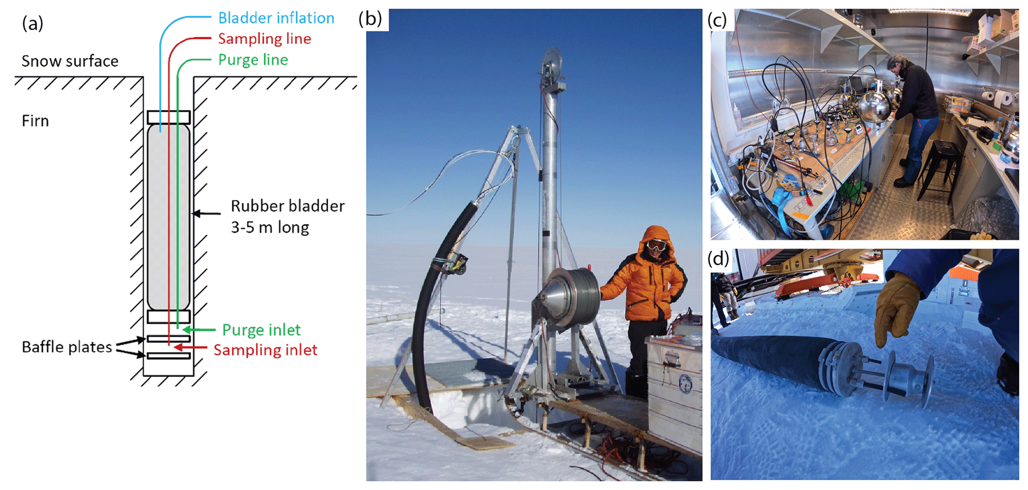
Figure 1(a) Firn-air-pumping schematic courtesy of Christo Buizert, (b) sampling in the field photograph courtesy of Anne Solgaard, (c) sampling of the pumped air at Little Dome C, Antarctica 2022, and (d) the purge and sampling inlets on the actual setup. The same equipment was used for the firn air-pumping in Greenland in 2018.
The CO2 and CH4 compositions of the firn air were monitored on-site during pumping to detect contamination issues, such as leakages in the system or sucking air from other stratigraphic layers, and provide a first determination of the age of the air. Four to seven flasks were filled at each depth to later measure the air composition in more detail. The total pumping time at each depth was 1.5 to 3.5 h, depending on the gas volume extracted.
In the field, the pumping conditions are stable throughout the diffusive zone, with similar, slightly decreasing concentrations of CO2 and CH4, mirroring the atmospheric increase over the past decades. The rapid decrease in CO2 and CH4 concentrations below 60.86 m are the first indications that the LIZ is reached, as the air suddenly ages rapidly, and diffusive mixing essentially stops. Soon after, the sampling system's flow rate decreases until filling the sampling canisters becomes impractical. That depth is then called the sampling close-off depth. At EastGRIP, it was reached at 66.61 m.
2.2 Results from the S6 borehole
Trace gas measurements in flasks filled during the firn air pumping at EastGRIP provide direct information about the location of the LIZ. We present the information obtained from the structure of δ15N, CO2, and CH4 mixing ratios in the open porosity of the firn. Moreover, CH4 measurements in the closed porosity were also retrieved from continuous flow analysis (CFA) of the deep firn and young ice, providing additional constraints on gas trapping in bubbles. Methane data in the open and closed porosity of the firn were used to constrain the evolution of pore closure at EastGRIP using a model of gas transport in firn (Witrant et al., 2012). We use a modified parameterization from Goujon et al. (2003) and from Mitchell et al. (2015) for our analysis. Due to the poor core quality, with seven to eight breaks per bag, there is a data gap between 72 and 75 m depth.
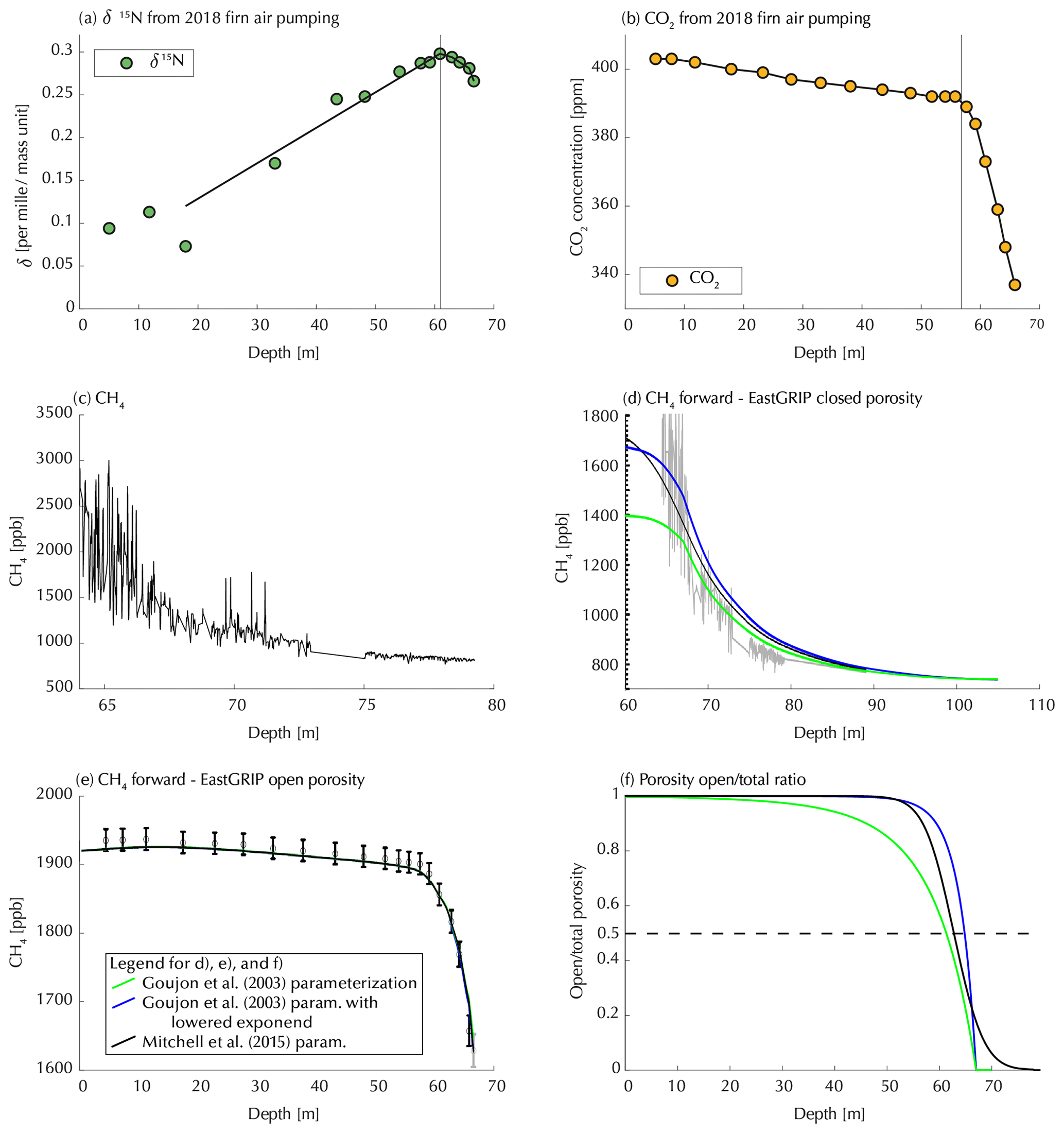
Figure 2 Measurements from the firn air-pumping campaign on the S6 borehole indicating that the transition of the diffusive to non-diffusive zone lies at around 61 m for (a) δ15N (not corrected for thermal fractionation) and 58 m depth for (b) CO2. (c) CH4 measured in the ice core, as a function of depth, around the bubble close-off. (d) Forward modeling of CH4 for closed porosity. (e) Laboratory measurements of CH4 in the air from the open porosity of firn (symbols) compared with IGE-GIPSA (Institut des Géosciences de l'Environnement and Grenoble images parole signal automatique) firn model results obtained with the two open- closed-porosity ratio parameterizations shown in panel (d) (the two model results are nearly superimposed). (f) Open- closed-porosity parameterizations used in the IGE-GIPSA firn model. Blue is for the usual parameterization using Eq. (6) in Witrant et al. (2012); green is for the exponential factor is reduced from 7.6 to 3.0.
2.2.1 δ15N isotopic ratios
The δ15N ratio is constant in the atmosphere over millions of years (Mariotti, 1983). It is therefore a great indicator of the fractionation processes happening in the firn. δ15N is reported using modern atmospheric air as a reference. First, mixing prevents isotopic fractionation in the convective zone, leaving δ15N at zero (same as the air). Then, in the diffusive zone, nitrogen isotopes fractionate: (1) due to gravitational settling, heavy isotopes are concentrated in the bottom of the firn, showing a linear increase in δ15N with depth. (2) Due to thermal gradients, heavy isotopes concentrate in the cold portion of the firn (Severinghaus et al., 1998). In Fig. 2a, at 12 m, we can see the recent summer atmospheric warmth just months before the pumping. Due to the atmosphere's virtually infinite reservoir, the nitrogen gas in the top dozen meters of firn, which is colder than the atmosphere in local summer, becomes fractionated with the heavy isotope δ15N becoming enriched (Severinghaus et al., 2001). On the other hand, the signal of the previous winter shows at 18 m, with a slightly depleted δ15N.
Finally, in the bottom section of the firn, the enrichment of δ15N stops, while there is still enough open pore space to extract air. This absence of further gravitational enrichment is evidence that vertical diffusion has stopped in this zone, although there is still a significant amount of open porosity. It is likely due to the layered nature of the firn; a dense layer is sealed off above a more porous layer from where air can be extracted, but this air is no longer in diffusive equilibrium with the open firn column. This last zone is the LIZ. The slight decrease in δ15N in the LIZ is due to global warming in the past 4–5 decades (Orsi et al., 2017). The maximum δ15N at 60.86 m gives an approximate value for the LID (Fig. 2a).
2.2.2 CO2 mixing ratios
Over the course of the past 2 centuries, the atmospheric CO2 mole fraction, commonly referred to as concentration, has almost doubled to approximately 420 ppm today (https://gml.noaa.gov/ccgg/trends/, last access: 27 June 2024). The depth range of the firn air pumping reaches a depth of 66 m, corresponding to around 385 years of snow deposition (Mojtabavi et al., 2020). In the diffusive zone, the firn air is in contact with the atmosphere and stays young; the CO2 concentration remains close to the atmospheric values and decreases slowly. In the lock-in zone, vertical diffusion is impeded, and the air ages as fast as the ice, which causes the CO2 concentration to decrease rapidly with depth.
The slope of the CO2 measurements from the S6 borehole firn air-pumping campaign significantly changes at a depth of 58 m (Fig. 2b). This change in slope suggests that the diffusivity is now rapidly decreasing and that the top of the LID has been reached.
The top of the LIZ is slightly different when using δ15N and CO2, and this difference is illustrated in a multi-site perspective in Table 2 of Witrant et al. (2012). In terms of gas transport, CO2 is more affected by diffusion rather than gravitation due to its important atmospheric time trend which induces a strong concentration gradient between the top and the bottom of the firn that diffusion tends to reduce. On the other hand, δ15N–N2 is more weakly affected by diffusion due to the absence of an atmospheric time trend and relatively more affected by gravitation, as well as advection, due to the sinking of firn layers. Together with the site-dependent abruptness of gas transport, a reduction around the LID and differences in the behaviors of CO2 and δ15N-N2 may occur. They may also respond differently to time variations in firn temperature or snow accumulation.
2.2.3 CH4 mixing ratios in open and closed pores
CH4 mixing ratios in the open porosity of the firn (dots in Fig. 2e) were measured at IGE (Institut des Géosciences de l'Environnement) and show an overall similar behavior to CO2, with a slope change in the 58–60 m depth range indicating the start of the LIZ.
In addition, the S6 firn core was measured by the CFA method for methane (Chappellaz et al., 2013; Faïn et al., 2022). Partial close-off results in the intrusion of modern air either since the time of core recovery or, in case the pores remain open until the time of measurement, during the measurements. Fourteau et al. (2019) observed correlated variations in the density, methane mixing ratio, and liquid conductivity in the LIZ of an Antarctic ice core, with positive spikes of methane induced by laboratory air reaching the center of the sample occurring in minimum density layers (Fig. 9 in Fourteau et al., 2019). Similar features were also reported in Mitchell et al. (2015) and Jang et al. (2019). Figure 2c shows a typical behavior of sharply decreasing CH4 variability with depth in the LIZ, reflecting the diminishing occurrence of sharp methane peaks due to modern air intrusions.
Layers with not fully closed pores can be found down to 71.5 m, although many pores are already closed at 66 m depth. Open porous layers alternate between impermeable layers, essentially hindering gas transport below the lock in depth. We note that such gas transport occurring at the centimeter scale in the CFA sample may not have an impact on the overall firn scale as the porosity in the surrounding layers is mostly closed. Methane data from CFA measurements in deep firn are too variable above 65 m to be used as a predictor of the LID but provide very good indications about full-air entrapment in the closed porosity which occurs above 72 m depth with some local layering effects.
2.2.4 Model constraints on open- total-porosity ratio
Progressive bubble closure during firn densification results in a gradual decrease in the ratio of open total porosity (values from one to zero) and the complete trapping of air into bubbles. Firn models simulating gas entrapment in ice usually represent the open- total-porosity ratio with a simple parameterization as a function of density (e.g., Goujon et al., 2003; Buizert et al., 2012). This ratio is difficult to measure, and available data show inconsistencies (Fourteau et al., 2019, Fourteau et al., 2020, and references therein). Here we adjust the open- total-porosity parameterization in a model of gas transport in firn (Witrant et al., 2012) in order to best simulate the CH4 concentrations in the closed porosity of the EastGRIP S6 core. Note that EastGRIP is a complex site, and constant temperature and accumulation for the stationary firn model might be offset for EastGRIP due to the effect of strain densification (Riverman et al., 2019; Oraschewski and Grinsted, 2021). The usual parameterization (Witrant et al., 2012; Eqs. 4 and 6; blue in Fig. 2f), adapted from Goujon et al. (2003) and also used in Buizert et al. (2012), results in CH4 concentrations that are too high in the model versus the data in the closed porosity of firn (Fig. 2d). In order to improve the model–data match, we modified the open- total-porosity ratio parameterization of Witrant et al. (2012) in Eqs. (4) and (6) by changing the exponential factor from 7.6 to 3.0 (green curve in Fig. 2f). A better match of the CH4 CFA data is obtained (Fig. 2d, in green), while the CH4 data in the open porosity are correctly modeled in both simulations (Fig. 2e) because a firn diffusivity tuning was performed for each simulation (Witrant et al., 2012). The beginning of the bubble closure moves significantly upwards, resulting in 50 % closed porosity at around 61.3 m (green in Fig. 2f) compared to around 64.8 m in the basic (blue in Fig. 2f) configuration.
2.3 Summary of Part I
We use δ15N, CO2, and CH4 (Fig. 2a, b, e) data from well-established methods to estimate the top depth of the LIZ. The depths we find are between 58 and 61 m, for the S6 borehole site. These depth ranges spread over 3 m, and with an annual layer thickness of 11 cm (Mojtabavi et al., 2020), this already results in an uncertainty of approximately 27 years. We also find two end-member scenario examples of how the porosity of the firn ice matrix changes from open to closed (Fig. 2d). Both end-members equally satisfy the firn air CH4 data, although the green curve is better tuned to the ice core CH4 concentrations. Together, these results show that firn air concentrations do not provide an unequivocal horizon for the LID or the evolution of closed porosity.
These results leave room for a more exact determination of where gases are locked into bubbles and where diffusivity approaches zero. The closing of pores is a physical property of the firn/ice matrix, and measurements of physical properties should help constrain the bubble closure process. In the following section, we investigate how optical scanning of the ice core can provide information on the bubble closure process and address these questions: is it possible to find the LID or COD using images obtained from the optical dark-field line scanner? Can we find a single solution for the gradual change from open to closed porosity? How sharp is this transition which later determines the range of gas ages in the ice?
By obtaining information about the physical properties of firn and ice from density measurements and line scan data, we aim to deepen our knowledge of how gases are trapped in the ice matrix. We introduce a new method to precisely confine the LIZ and thus shine more light on the firn–ice transition. We use this method to also obtain insight into the transition from open to closed porosity.
3.1 Density measurements from four Greenland ice cores
Density measurements have been conducted on the S2, NEGIS, and NEEM ice cores which are all located in central Greenland, and the density data have not been published yet. The density increase follows a similar trend in all three cores (Fig. 3a). The NEEM ice core starts higher, and density increases are slower than in the other two cores. This trend is due to different boundary conditions at its location 400 km away from the other two cores on the other side of the Greenland ice divide. The S2 and NEGIS cores are located close together (see site location section), and both exceed the value of 790 kg m−3 at around 60 m depth.
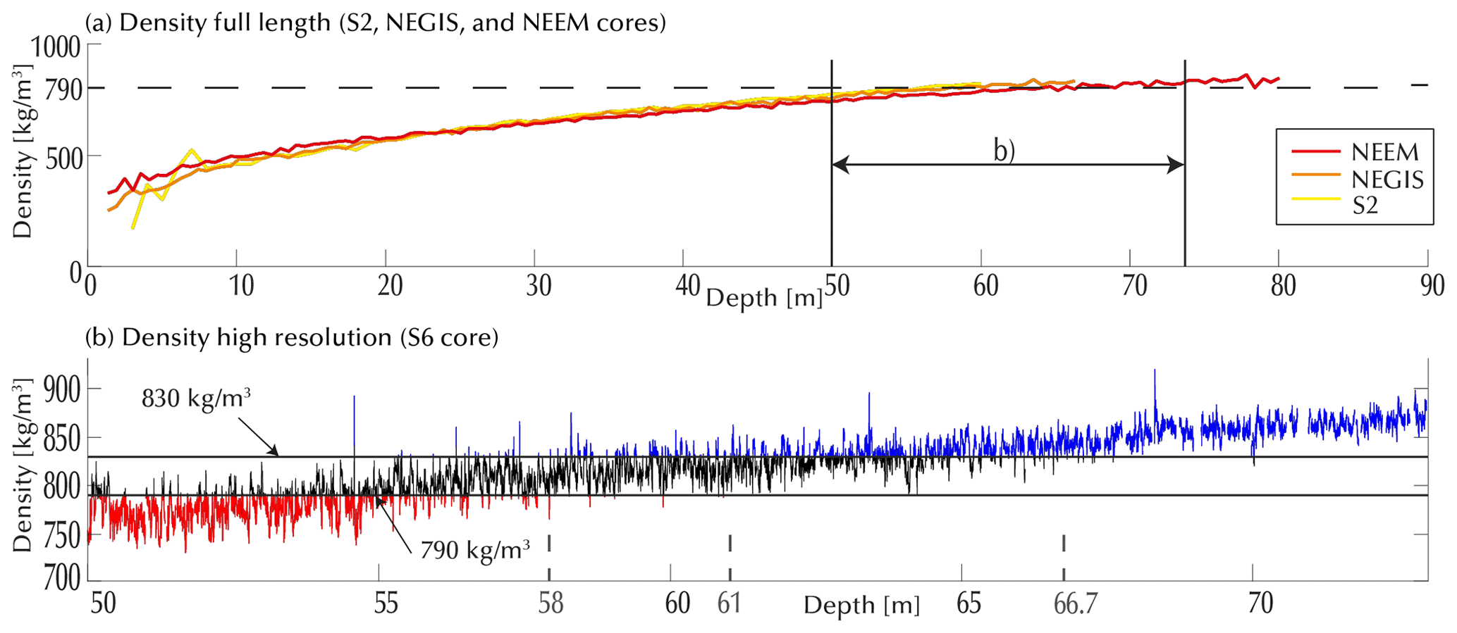
Figure 3(a) Density of the S2, NEGIS, and NEEM ice cores as 1 m, 55 cm, and 55 cm averages, respectively, measured by weighing in the field. (b) High-resolution density of the S6 ice core derived from micro-CT measurements. Values below 790 kg m−3 are in red, values above 830 kg m−3 are in blue, and values in-between are in black. Depth results from Part I are in gray on the x axis.
In general, the close-off zone can be defined by density values between 790 and 830 kg m−3 (Schwander and Stauffer, 1984). At a density of 830 kg m−3, the material is defined as ice, and bubbles are believed to be completely closed off.
High-resolution density data from micro-CT scanning are available in a depth range from 50 to 73 m conducted on the S6 core (Fig. 3b). With depth, the density increases and exceeds 830 kg m−3 for the first time at 54.58 m depth. This depth corresponds to a melt layer found in the EastGRIP core (Westhoff et al., 2022). Below this, we find three peaks at 56.33, 57.42, and 58.3 m depth which are high-density layers and could potentially be a seal for gas diffusion. Between approximately 50 and 67 m depth, density values lie between 790 and 830 kg m−3, suggesting this to be the LIZ. Below this depth, essentially all density values correspond to bubbly ice.
3.2 Visual stratigraphy
3.2.1 Line scanning ice cores
The line scanner camera images a polished, 165 cm long ice core slab from above, while it is being illuminated from below (Svensson et al., 2005; Faria et al., 2018; Westhoff et al., 2020). As the light travels through the firn/ice, it can be reflected on various features, such as snow and firn grains, core breaks, bubbles, dust-rich layers, and others. In ice from the Holocene period, corresponding to the upper approximately 1100 m of the EastGRIP ice core (Mojtabavi et al., 2020), the main causes of reflection, refraction, and scattering are air bubbles within the ice and core breaks (Westhoff et al., 2022). These features appear bright in the line scan images. The EastGRIP line scan images are provided by Weikusat et al. (2020).
Between firn and ice, there is an inversion of bright and dark sections (Westhoff et al., 2022). Low-density firn and snow can be seen as grains embedded in a matrix of air; the grains thus appear bright, as they are small objects scattering light. In dense bubbly ice, the picture is reversed; we have bubbles embedded in an ice matrix which is now the bright object scattering light. In the transition from firn to ice, we see mixed elements of both appearances (Fig. 4).
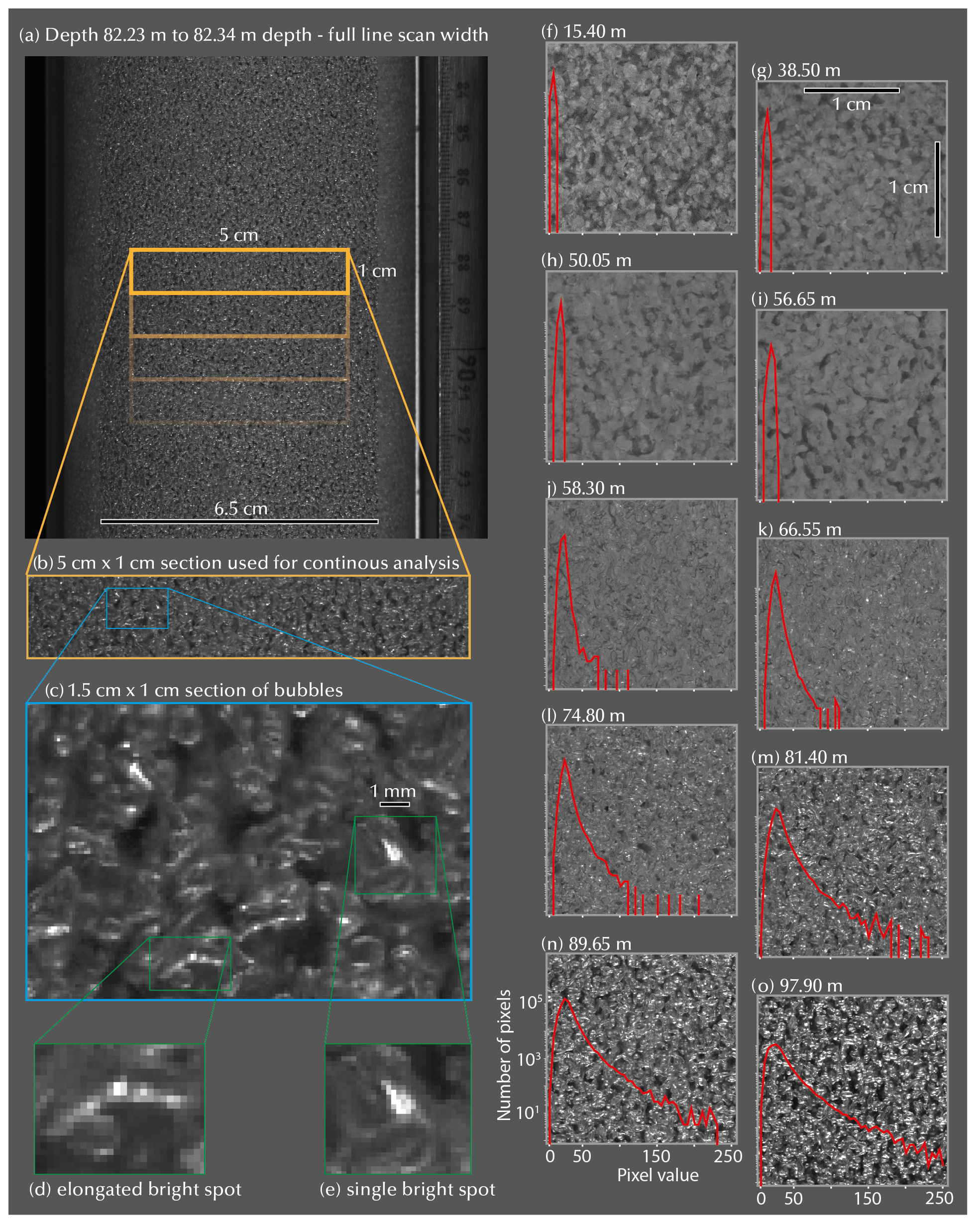
Figure 4 (a) An 11 cm section of a 165 cm long line scan image in its full width from 82.23 to 82.34 m depth. The 5 cm × 1 cm sections used for the bright-spot and bubble analysis are indicated in yellow and in panel (b). (c) Close-up of the ice and bubble structure (1.5 cm × 1 cm). (d) An elongated bright spot. Depending on the pixel value thresholding, this could be counted as one or multiple bright spots. (e) A single bright spot made up of many pixels. This is used as a proxy for counting bubbles. (f–o) Some 2 cm × 2 cm example images across the upper 100 m, with the scale in panel (g). In red is the log-scale pixel distribution of image sections, with the scale in (n) and with the same scale for the images in panels (f) to (o). Note that all images have been brightness-enhanced for better visualization. Spots appearing bright to the eye have pixel values above 60.
3.2.2 Bubble and pixel value analysis
The analysis of pixel brightness intensities from the line scan images is commonly done on recent ice cores (e.g., Svensson et al., 2005; Morcillo et al., 2020; Stoll et al., 2023). We investigate the uppermost section of the EastGRIP ice core, i.e., from 13.75 m below the surface to 99.40 m, whereby we measure the intensity values for pixels (px) on 1 × 5 cm2 increments (Fig. 4a, b).
The lighting from below the ice core slab is refracted and bundled on rounded solid–gas interfaces, causing bright reflections, white spots, or, using the terminology from Morcillo et al. (2020), bright spots (Fig. 4c, d, and e). We count the bright spots as a proxy for the number of bubbles in our samples. Bright spots are clusters of bright pixels in the image (Fig. 4e). To analyze the bright spots, we convert the grayscale image (pixel range from 0 to 255) to a binary image (0 or 255), and we use three different thresholds, namely 60, 150, and 250. Depending on the threshold, the number of bright spots, a proxy for bubbles, changes (Fig. 4d). The choice of 60 is arbitrary and based on what appears bright to the eye. Similar results were obtained for values of 50 or 70 but are not shown here. The values of 150 and 250 show similar trends yet with a much lower amplitude. To convert from the bright spots to a bubble proxy, we do not use the method of Ueltzhöffer et al. (2010), due to complicated 3D effects from our thick line scans, nor do we use a blur function (or similar) to correct for gaps in bright pixels belonging to the same bright spot that might therefore overestimate the number of bubbles. Yet, our analysis is simple and sufficient to detect the first formation of bubbles, and it also makes layering visible within the LIZ.
Therefore, 1 cm in our line scan sample is represented by 186 px, with each 1 × 5 cm2 increment thus having a size of 186 by 930 px. The pixel values range from 0 to 255, representing 256 possibilities. The value of the single lowest/highest pixel inside this 186 by 930 px area is then used to describe the minimum/maximum value of this depth. The OLID is based on the changes in the minimum and maximum pixel value per increment with depth.
For the upper 100 m of the core, we show 10 selected 2 cm × 2 cm examples (Fig. 4f to o). Here the change from firn to ice is optically visible and elaborated on in more detail in Appendix A. The distribution of the pixel values within one sample changes with depth, as shown by the red curves in Fig. 4f–o, which are plotted on a log scale. Figure 4f–i have a very narrow distribution in the lower pixel ranges. With the first appearance of bright spots, this distribution suddenly broadens in Fig. 4j and progressively broadens with depth.
3.2.3 What causes these bright spots in our images?
Lens effects on the gas–solid interface of bubbles in the ice matrix cause the bright spots we see. To understand the occurrence of these features, we have to look at the termination of the pore space structure into isolated clusters and eventually into individual spherical bubbles, which can be seen as a percolation transition (Li et al., 2021). At this transition, the pathways disintegrate and form individual clusters, i.e., bubbles.
If we think of the pore space as a pore network with many redundant connections, then, above a certain density, the connections gradually disappear, and isolated clusters of different sizes are formed, while a permeable network also remains. With depth, i.e., in the process of metamorphism, many connections are cut, and the permeable clusters become increasingly smaller. The LID is the horizon where pore clusters become disconnected from the surface. Below that, the isolated pore clusters disintegrate down to the smallest units, namely bubbles (i.e., closed-off bubbles), upon further compaction. This percolation transition is superimposed on the stratification, i.e., layers with different percolation states alternate. Therefore, large percolation clusters can still be found below the LID, and air can be extracted from them.
If we assume that bright spots are created by singular/spherical bubbles, then we do not expect them to occur at the beginning of the percolation transition but only when most connections are closed off. It therefore makes sense that we do not see the bright spots at the first-occurring closed porosity (around 50 m) but further down.
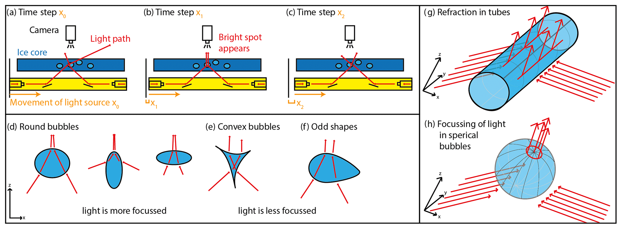
Figure 5(a–c) Line scan setup with a fixed camera and ice core and a moving light source (yellow). In certain settings, the introduced light will refract and bundle, causing bright spots (b). The amount of light bundling is a geometric effect dependent on the bubble shape, e.g., (d) rounded bubbles, (e) convex bubbles, or (f) other shapes. The amount of bundling/focusing is also dependent on the 3D bubble shape as tubes bundle less often (g) than spheres (h).
Our analysis shows a sudden appearance of bright spots below a depth of 58.3 m (Fig. 4j). We interpret these bright spots to be a geometric effect of rounded bubbles causing refraction of the injected light, bundling it, and causing this bright appearance in the image (Fig. 5). With the correct bubble shape, these bubbles will then appear bright as the light source moves below the ice core (Fig. 5a to c). We assume that these bright spots only occur once bubbles are rounded or have an ellipsoid shape, are sealed off, and trapped in the ice matrix (Fig. 5d, h). Clusters or tubes of bubbles would not create bright spots with such intensity (Fig. 5g). Odd shapes of bubbles will most likely not lead to such an intense bundling of light and will therefore appear less bright (Fig. 5e, f), while spherical bubbles can focus the light and thus generate a brighter appearance in the images (Fig. 5h).
3.3 Visual-stratigraphy-derived lock-in depth
The line scans are grayscale images with pixel brightness values ranging from 0 to 255, resulting in 256 options for one pixel. The minimum pixel values (Fig. 6a; yellow line) of each 1×5 cm2 increment remain relatively constant over the upper 100 m of the EastGRIP ice core. This ensures constant camera settings without any adjustments made to the brightness. From the first processed ice core section (13.75 m) to 58 m, the minimum (yellow), median (red), and maximum values (brown) do not vary much, and maximum values are low (Fig. 6a). We see a small peak at 50 m and two troughs at around 54 and 58 m. Below 58 m, we see a trend of linearly increasing maximum pixel values (Fig. 6a; dashed brown line) from 58 to 85 m. During this increase, the median value (red) remains at a constant value, indicating that there are very few bright pixels in one increment (Fig. 4j, k, l). Below 85 m depth, the maximum values remain at 255 over several meters. We identify a drop at around 90 m, and then the value returns to a maximum of 255. During the increase in pixel values below 58 m depth, we identify peaks, indicating some sort of layering in this section (discussed later). Figure 6a has a resolution of one 1×5 cm2 sample every 55 cm (in the center of every bag).
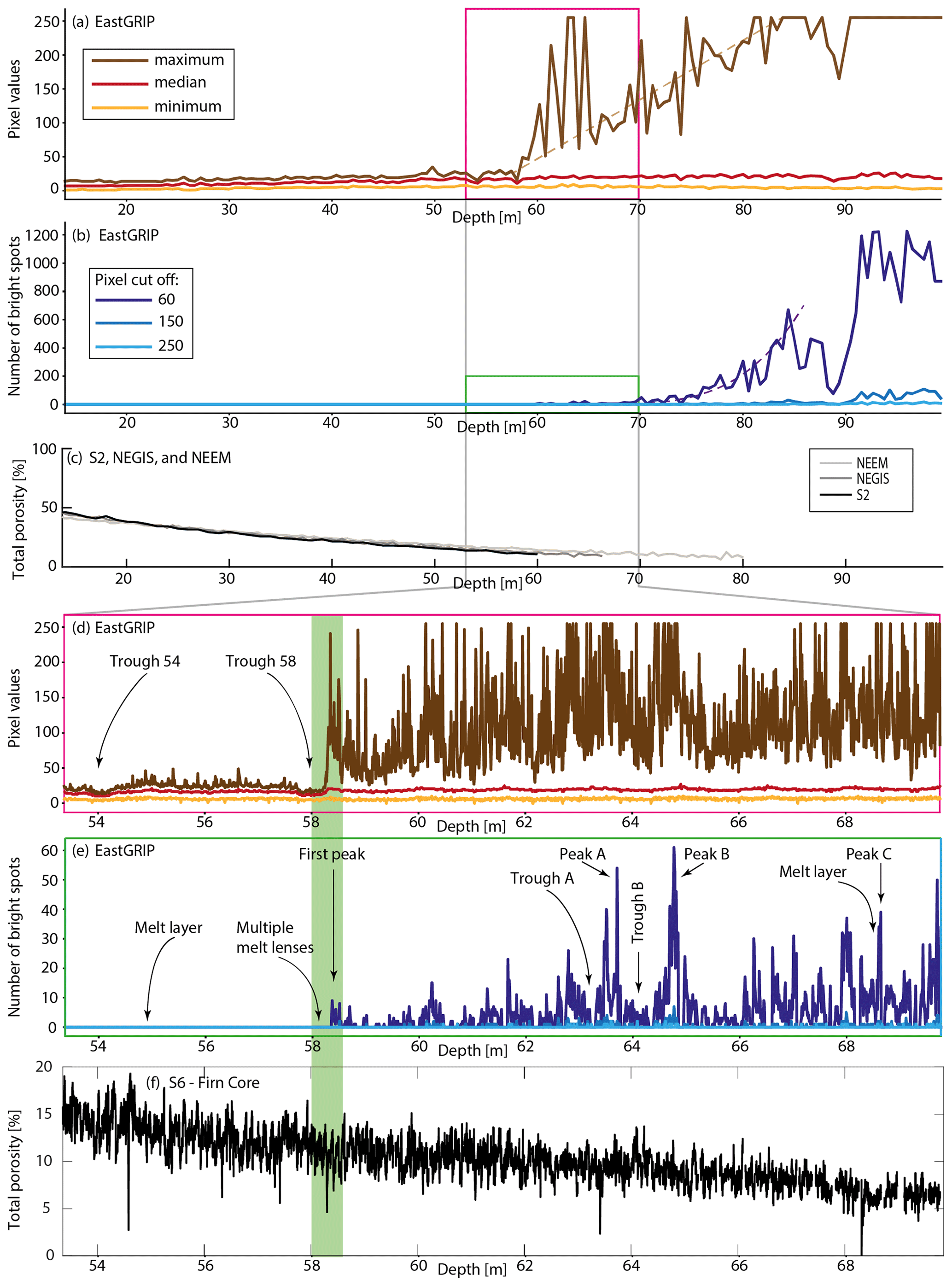
Figure 6Depth of investigation from 13.75 to 99.40 m below the surface with one measurement every 55 cm (a, b). Detailed analysis from 53.35 to 69.85 m with continuous measurements every centimeter (d, e). Our analysis locates the OLID at 58.30 m depth. We find a linear increase in maximum values in panel (a) and a roughly exponential increase in bubbles in panel (b) (dashed lines). Both panels (d) and (e) show a sudden appearance of bright spots below 58.30 m, with the layering clearly visible in panel (e). (c) Total porosity calculated from density data of the S2, NEGIS, and NEEM ice cores and (f) total porosity from micro-CT density data of the S6 ice core (Freitag and Westhoff, 2024. The full high-resolution S6 profile will be published later.).
Figure 6b is an attempt to determine the number of bubbles from the bright-spot proxy. Between 58 and 85 m, we see an exponential increase (dashed purple line) in the bright spots. Between 85 and 90 m, we find two drops to very low bright-spot numbers and then a sudden increase to between 800 and 1200 bright spots per 1×5 cm2 image, where it remains constant with depth. The number of bright spots is strongly dependent on the threshold chosen, but the trend is similar yet hard to see in the medium and light blue curves.
In the interval between 53.35 and 69.85 m (Fig. 6d; pink box in Fig. 6a), we inspected the bubble closure in detail with a 1 cm resolution, as opposed to a 55 cm resolution in Fig. 6a and b. The drops of all pixel values at around 54 and 58 m (trough 54 and trough 58, respectively) have a width of approximately 30 cm. Below the last trough, at 58.30 m, the maximum pixel values (brown) greatly increase, almost reaching the maximum of 255. Higher maximum pixel values than the average of the shallow depths represent the first appearance of bright spots in the line scan images (see also Fig. 4e). The detailed inspection does not show a gradual increase in the maximum pixel values but rather multiple peaks and troughs representing layers containing more and fewer bubbles.
Figure 6e (green box in Fig. 6b) also shows the sudden appearance of bright spots at a depth of 58.3 m. The peaks in Fig. 6d–e align, but peaks are more visible in Fig. 6d. The number of bright spots does not show a gradual increase but rather, just like Fig. 6d, multiple peaks and troughs. A prominent example of this alternation is peak B (Fig. 6e), where we find a prominent trough followed by a peak.
From the density data, we calculate the total porosity of our ice core samples (Witrant et al., 2012; Eqs. 2 and 3). The S2, NEGIS, and NEEM total porosity gradually decreases over the measured depth (Fig. 6c). The high-resolution total porosity data, derived from micro-CT density data from the S6 core, show four cases of porosity greatly dropping between 54 and 59 m depth (Fig. 6f). A very dense layer at exactly 58.3 m depth, corresponding to very low porosity, coincides with the depth at which we find the first bright spots. This could be the impermeable layer, below which diffusion is increasingly limited.
3.4 Stratigraphic layering in the lock-in zone
Layering in the LIZ can influence bubble closure (e.g., Blunier and Schwander, 2000; Mitchell et al., 2015; Fourteau et al., 2019; Jang et al., 2019). This idea motivated Birner et al. (2018) to establish a 2D model which includes layering in order to better reproduce the lock-in of air bubbles. With the line scan images of the EastGRIP firn section, we now have a unique chance to further investigate this layering. We also investigate the influence of melt layers around the LIZ in Appendix D.
The pore network is not homogeneous, as the temperature gradient metamorphism in the upper snowpack already introduces anisotropy into the structure. The strangulation, i.e., reduction in the gas exchange between layers, does not progress continuously with the reduction in the porosity but rather collapses in phases. One of these phases seems to be reached when the impermeable cluster collapses and single pores separate.
Figure 6a shows that between 58 and 85 m depth, more and more layers contain these bright spots until, below 85 m depth, all image increments have at least one bright spot, suggesting that all layers are impermeable. The data used for Fig. 6a–b are obtained from one 1×5 cm2 increment every 55 cm. Therefore, the plot does not show an average of many values but one single snapshot of that depth. We see strong variations in the maximum pixel values (legend in Fig. 6) as we do not always measure a layer with rounded bubbles and bright spots.
Figure 6d–e show the variability during the lock-in. The maximum pixel brightness (Fig. 6d) covaries with the number of bright spots (Fig. 6e). Thus, some layers do not have these rounded, ellipsoidal, and sealed-off bubbles, while others do. An exact correlation of the bubble number (Fig. 6e) with density (Fig. 6f) remains a challenge, as the analysis was conducted on different ice cores, namely EastGRIP and S6, respectively.
From the visual stratigraphy data, the (optical) lock-in seems to appear suddenly. Yet we must keep in mind that a small change from an odd shape to rounded bubbles can cause a significant change in the optical appearance (Fig. 6d to f; green bar). The number of bright spots (Fig. 6e) shows a small increase at first, and some layers with more bubbles and others with fewer bubbles are visible. This indicates layering as not all odd-shaped bubbles or clusters transform into spherical bubbles at the same depth. When the bubble number drops to zero, the reason is mostly missing data due to core breaks. Yet the height of the peaks, i.e., the number of bright spots, varies throughout the LIZ.
3.5 Ice core porosity derived from visual stratigraphy
3.5.1 Methods
When the firn porosity is still fully open, e.g., at a depth of 44 m, the firn and the open pores have pixel values around 15 and 10, respectively (see Fig. B1a in the Appendix). As bubbles are isolated, their edges become brighter and gradually exceed a pixel value of 20 (see Fig. B1b to c), while the black patches in the images remain at a pixel value of 10 (see Fig. B1). Thus, the edges of the bubbles become more distinct. With increasing depth, the air–ice interfaces appear even brighter, gradually exceeding a pixel value of 20, and single bright spots become visible (see Fig. B1d).
3.5.2 Results
From the fraction of open total porosity (Fig. 2f), we calculate the fraction of closed to total porosity, namely closedtotal opentotal. The two end-member states are displayed in green and blue, and the Mitchell et al. (2015) parameterization is in black (Fig. 7). Results from Part I suggest 100 % closed porosity at a depth of 67 m (dashed vertical line in Fig. 7), using the Goujon et al. (2003) parameterization, and a more gradual approach to 100 %, using the Mitchell et al. (2015) parameterization.
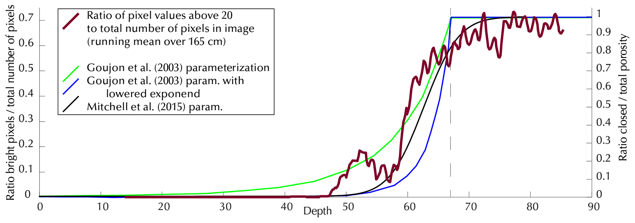
Figure 7Closed total porosity calculated from open total porosity (Fig. 2b) in green and blue. Percent of the image covered by pixels greater than 20 in is shown in black. Running means over one line scan sample (165 cm) are to reduce the brightness fluctuations within one sample.
Using the line scan images, we calculate the percentage of pixel values exceeding 20 of the total image. Above 40 m depth, almost all pixels have values below 20; i.e., the ratio of bright pixels to total pixels is 0 % (black curve in Fig. 7). At a depth of around 46 m, the ratio of brighter to total pixels increases slightly and sharply increases at a depth of 58.3 m. The ratio gradually plateaus at a depth of 70 m at values around 65 % to 70 %. Due to the nature of the line scan images, a ratio of approximately 0.7 is not exceeded and can be considered the maximum.
3.5.3 Discussion
Using a pixel cut-off of 20 brightness units is a simple way to describe a more complicated process. As the metamorphism of firn grains to ice crystals takes place, their structure significantly changes. Firn, in the line scan images, appears as a homogeneous surface with dark patches in between the open pores (Fig. B1). Closed pores appear differently, i.e., brighter, with sharper brightness contrasts and with apparently more structure (Fig. B1b; just above the star). This closure adds a third feature to the visual stratigraphy image, which now contains ice, open pores, and closed pores. This increase in the structural complexity can be seen in Fig. B1c as thin lines in the line scan image. The appearance of ice, without open pores, is visible in the absence of any homogeneously bright image patches, i.e., former firn. While the process of transforming open pores to closed pores is a complex process, it can easily be described by analyzing the number of pixels in an image exceeding a value of 20.
The ratio of pixel values above 20 to the total number of pixels (black line in Fig. 7) shows the trend of how the firn/ice–air interfaces are changing due to pores becoming closed off and thus becoming more reflective for the light of the line scanner. The pixel ratio (black curve) has a strong similarity to the ratio of the closed total porosity (green curve), and both follow the same trend. The ratio of closed total porosity increases with depth until all pores are closed off at a depth of approximately 67 m. This process is more gradual, over many meters around 67 m in the line scan data (black), and shows a similarity with the work of Mitchell et al. (2015), who measure the closed porosity directly.
Although the line scan data are shown as a running mean average over 1.65 m, we still see layering and changes above the annual variability. This indicates further layering in the firn, e.g., with more closed-off bubbles from 50 to 55 m and fewer from 55 to 58 m depth (Fig. 7).
3.6 Summary of Part II
Density measurements and visual stratigraphy data can reveal more details about the firn–ice transition. Here we combine data from the S6 and the EastGRIP core. High-resolution density data show the presence of high-density, or low-porosity, layers exactly at the depth where airflow starts to reduce to a minimum during the firn air-pumping campaign. Visual stratigraphy pinpoints the exact depth at which a change in physical properties causes the appearance of bright spots. This sudden appearance of bright spots is associated with a change in the firn/ice to air boundaries and the shape of bubbles. The sudden appearance is not connected to a change in the ice core processing procedure, such as microtoming the surface (see Appendix C). The number of bright spots as a function of depth indicates a layering in the firn and ice, meaning that some layers favor containing more bright spots, i.e., closed-off bubbles, compared to others.
By analyzing the change in the appearance of firn and pores with depth, we find a simple correlation between the closed pore space and image brightness. Using this correlation, we can add more details to the transition of open closed porosity throughout the firn–ice transition.
Including physical property data with the traditional methods of defining the LIZ can add details and can further increase our understanding of the firn–ice transition.
All the data presented in this work indicate that the transition between the diffusive and non-diffusive zone in the EastGRIP area occurs between 58 and 61 m. δ15N suggests a depth of 61 m (Fig. 2a), and CO2 and CH4 suggest a depth of around 58 m (Fig. 2b and e, respectively). The OLID suggests a depth of 58.3 m (Fig. 6d). Thus, all methods, including the optical method, agree well.
The ice from 58.3 m depth was deposited in the year 1681 CE (Mojtabavi et al., 2020), i.e., 338 years before the 2017 drilling. Including a typical mixing delay of 10 to 50 years at Greenland sites (Schwander et al., 1988), the gas–ice age difference ranges from 288 to 388 years. The Mitchell et al. (2015) parameterization and the adjusted Goujon et al. (2003) parameterization agree well with these values, with a delta age of 345 years and 350 years, respectively (Fig. 8).
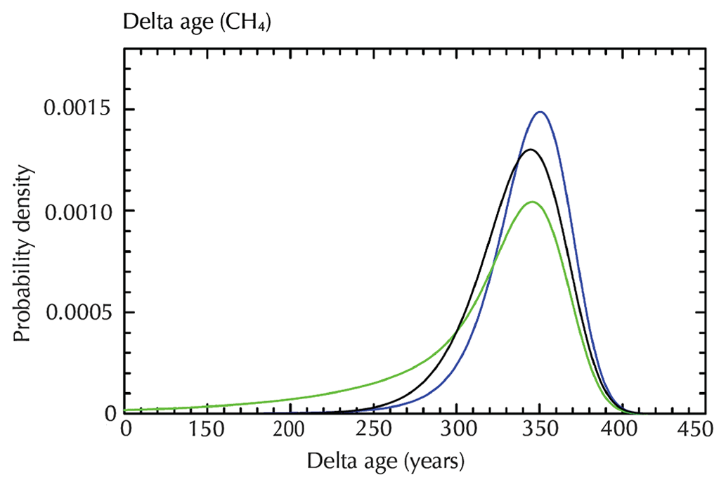
Figure 8Delta age distributions using different parameterizations (see Fig. 2). The different parameterizations discussed throughout this paper all result in a delta age of around 350 years.
In this work, we have presented a method based on the physical properties of the ice core to obtain information about the LIZ and the transition from diffusive to non-diffusive zone and to increase our understanding of open closed porosity. The method works accurately and is in agreement with the traditional methods that obtain results from firn air-pumping campaigns in boreholes. It further offers the advantage of resolving centimeter-scale variability, which is beneficial to better understand the impact of firn stratification on gas entrapment. We investigated the EastGRIP area, as we had the best data coverage from this region. We hope to use this method on sites around Greenland and Antarctica in the future.
The importance for future line scan processing is to have a continuous camera setting that is unchanged throughout the upper 100 m of the ice core. Hereby, two scans should be performed, namely a dark setting, to make use of our method, and a bright setting to make the images analyzable by eye.
5.1 RECAP, coastal Greenland
The RECAP ice core, from eastern coastal Greenland, is the only other core for which visual stratigraphy data are available from the ice sheet surface to below the firn–ice transition. When trying to analyze this core, we faced many challenges, such as changes with respect to camera settings, numerous melt layers disturbing the light reflections, and strong changes in brightness between summer and winter layers. A first test shows that it is possible to use this method on the RECAP ice core, despite the challenges. We plan to analyze the RECAP core in the future, together with other ice cores which will have been line-scanned by then.
5.2 Beyond EPICA, Antarctica
The Beyond EPICA (European Project for Ice Coring in Antarctica) ice core is currently being drilled. Processing has not taken place yet, and we hope to acquire line scan images throughout the firn section. With these images, we can then test the here-presented method on an Antarctic ice core, where conditions are expected to be more similar to EastGRIP than to RECAP, as we do not expect melt layers.
Line scan images provide a 2D picture of the structure of the ice cores. The focus depth is set to a few millimeters below the ice core's polished surface. While these 2D images cannot provide a full 3D reconstruction such as a computer tomography scan (e.g., Freitag et al., 2013, or Lipenkov, 2018), it does reveal some structures, and we can get a hint of what the 3D structure could look like. Experience in using the line scanner reveals that when using the camera settings, as done in Fig. 4, we have approximately half a centimeter in focus, which is then visible in the image. As light is introduced at an angle from below, the ice below and above our focus depth remains invisible.
Figure 4a (depth below the ice sheet surface of 15.40 m) shows one of the first samples that was scanned. We see firn grains in different shadings of gray, and voids are scattered across the 2 cm × 2 cm image. From Fig. 4a–d, the firn grains remain bright, and the voids connect to more elongated structures.
Our image analysis shows a significant change in the appearance of texture at 58.30 m depth (between Fig. 4d, e). This change is represented by the first appearance of white spots in the images, which provide evidence for the first formation of rounded continuous ice–air interfaces, i.e., trapped air bubbles. The lighting from below the ice core slab is reflected on these rounded solid–gas interfaces, thus causing bright spots.
Further analysis of sections below the firn–ice transition shows an increase in bright spots, which reveals the gradual closure of air pathways. As this is a 2D analysis, connections into the y axis (into the page) can easily be missed. Yet, analyzing the x and z axes (lateral extension and depth axis, respectively) gives an idea of the distribution and scale of air pathways.
While Fig. 4e shows bright spots, these are optically not visible as closed bubbles but could also be pathways evolving into a rounded shape. The first definite evidence of closed bubbles can be found at a depth of 66 m, where, with a 2D appearance, some bubbles appear fully enclosed (Fig. 4f).
At a depth of 74.8 m (Fig. 4g), we can identify closed bubbles, together with tubes of bubbles, which are still connected. These tubes and bubbles decrease in size, causing a further closure of pathways within the ice (Fig. 4h).
At a depth of 89.65 m (Fig. 4i), all bubbles are fully closed off, without any sub-centimeter-scale pathways on the x and z axes. Pathways may still appear in the y direction. While bubbles form, the space of the image occupied by dark areas, i.e., clean ice, starts to increase.
When the firn porosity is still fully open, e.g., at a depth of 44 m, then the firn and the open pores have pixel values around 15 and 10, respectively (Fig. B1a). With depth, the black patches in the images remain at a pixel value of 10 (Fig. B1). As bubbles close off, their edges become brighter and gradually exceed a pixel value of 20 (Fig. B1b to c). At increasing depth, the air–ice interfaces appear brighter, exceeding a pixel value of 20, and single bright spots become visible (Fig. B1d). The pixel value of 20, therefore, seems to be a reasonable cut-off for when firn transitions to ice and when the reflectivity increases. Note that these values are dependent on the camera settings and need to be adjusted for other ice cores and/or sets of images.
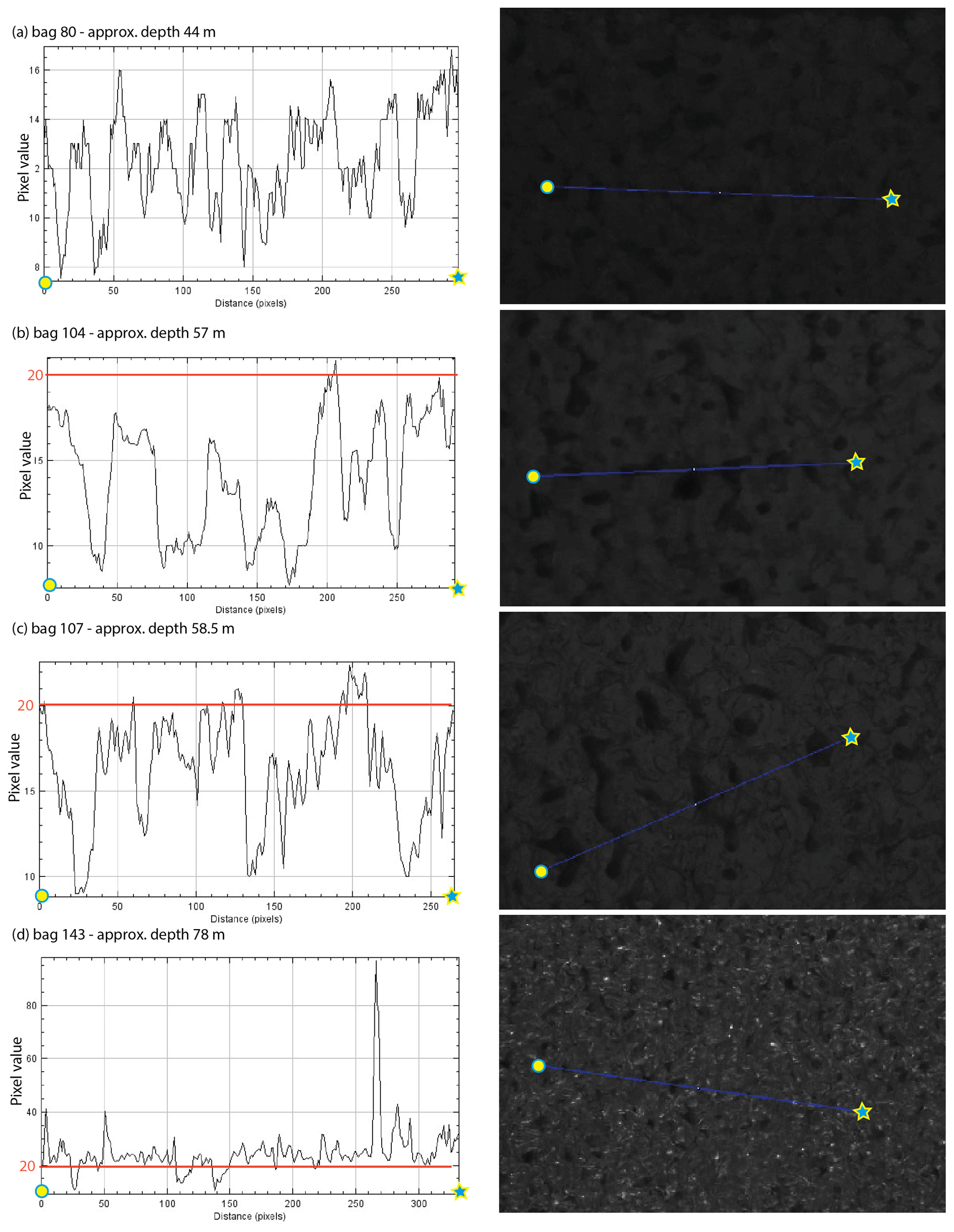
Figure B1The change in the brightness appearance with depth. (a) Above the firn–ice transition, (b–c) the transition, and (d) below the firn–ice transition. The left-hand side shows the brightness profiles from the blue lines on the right-hand side. The image width is approximately 2 cm.
In an early stage of this work, the sudden appearance of bright spots in the line scan data was allocated to a change in ice core processing, i.e., starting to microtome the ice core surface before scanning it. We investigate 1 × 5 cm2 images over the optical LID to find that the appearance of bright spots is an effect of metamorphism and not of a change in ice core processing procedure. The transition to locked-in bubbles, and our proposed OLID, appears in Fig. C1b and c at 58.3 m depth. Between Fig. C1a–b and d, we see a distinct difference in the appearance as firn-to-gas boundaries become more distinct. Figure C1c shows both appearances in one image; on the left we see an appearance similar to Fig. C1b and on the right similar to Fig. C1d. As we see both appearances in one image, the effect of bright spot occurrence cannot be due to the start of microtoming the surface but is an effect of metamorphism.
The black pixels in Fig. C1c and d represent over-saturated pixels; i.e., they are those detected by our bright-spot analysis.
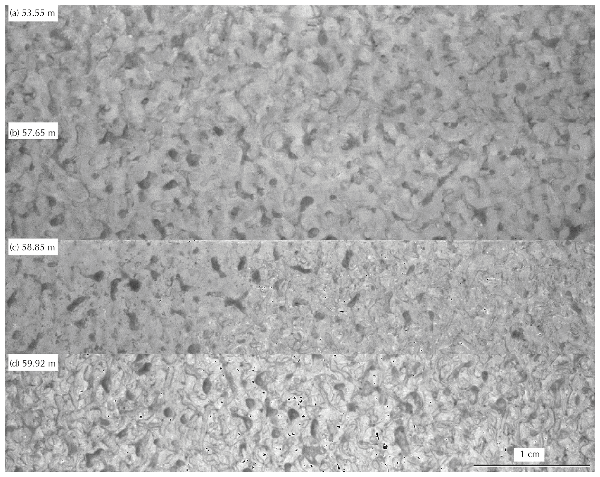
Figure C1Brightness-enhanced images over the optical LID (EastGRIP). Panels (a) and (b) show the appearance of firn without bright spots (here converted to black). Panel (c) shows the transition, and panel (d) shows multiple bright spots and clearer firn–gas interfaces.
The study by Westhoff et al. (2022) provides an overview of melt events in the EastGRIP ice core. In the following, we analyze the melt layers and melt lenses in the proximity of the LID. Blunier and Schwander (2000) state that “All mixing processes are strongly influenced by the presence or absence of icy layers resulting from surface melting during summer”. In the 16 m around the OLID (Fig. 6d, e), we find two melt layers in total at 54.80 and 68.60 m depth. The upper one should be treated with caution, as it is located next to a core break and could be an imaging artifact rather than a true layer (top of bag 99; Fig. D1; Westhoff et al., 2022). In the following 30 cm below this melt layer (bag 99), we find the section with significantly darker line scan images (i.e., lower pixel values compared to Fig. 6e; trough 54). Darker layers such as these have been influenced by summer surface melting or pre-melting (Dash et al., 2006).
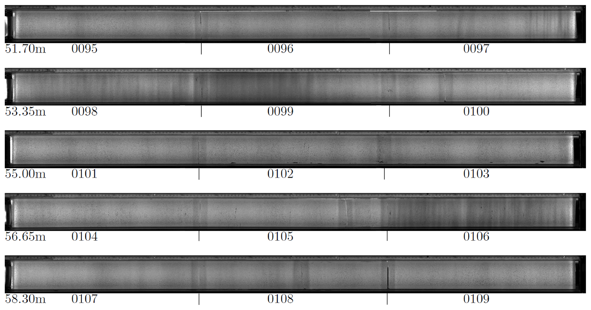
Figure D1Bags 95 to 109 showing brightness variations in the line scan images and melt layers (from overview booklet; Westhoff et al., 2019).
The ice at 55 to 58 m depth is characterized by the occurrence of 11 melt lenses in total. These are small melt patches with a horizontal extent that is shorter than the core width, i.e., less than 10 cm. Four of these lie between 58.00 and 58.16 cm depth (Fig. 6e), just above the LID and inside the darker line scan image section (bag 106; Fig. D1). Melt lenses are evidence of strong surface melting, most likely during summer, and thus an alteration of the physical properties of the snowpack. This alteration can work as a block for vertical diffusion and thus enhance the formation of the first bubbles below this depth.
The influence of a melt layer at 68.6 m is visible in our data (Fig. 6e) but not to an outstanding degree. Just below the melt layer, we find a layer containing many bubbles, which is probably an effect of reduced diffusivity due to the solid, bubble-free ice layer above. Yet this peak (peak C; Fig. 6e) is equally as high as other bubble-rich layers and thus indicates that melt layers must not necessarily cause an outstanding effect on the bubble close-off. A reason for this uncertainty could be the limited size, 10 cm width, of the ice core and image and therefore the inability to quantify the extent of the melt layer over more than 10 cm.
Delta 15N, CO2, and CH4 data are in the Supplement of this paper. Modeled CH4 open- and closed-porosity data are available on request from Xavier Faïn (xavier.fain@univ-grenoble-alpes.fr) and Patricia Martinerie (patricia.martinerie@univ-grenoble-alpes.fr). The delta age parametrization is available on request from Patricia Martinerie (patricia.martinerie@univ-grenoble-alpes.fr). High-resolution density data from 50 to 73 m of the S6 core is available at http://doi.org/10.17894/ucph.fa813160-65d0-489f-8f4d-f9c728f44650 (Freitag and Westhoff, 2024). The full dataset will be published by Johannes Freitag (Alfred Wegener Institute, Bremerhaven, Germany; johannes.freitag@awi.de). Density data from NEEM, S2, and NEGIS core are available on request from Anaïs Orsi (aorsi@eoas.ubc.ca and anais.orsi@lsce.ipsl.fr). The line scan data set from EastGRIP from Weikusat et al. (2020) is available on PANGAEA (https://doi.org/10.1594/PANGAEA.925014).
The Python script for the pixel count analysis is available in the Supplement of this paper.
The supplement related to this article is available online at: https://doi.org/10.5194/tc-18-4379-2024-supplement.
JW came up with the initial idea of using the optical method, wrote most of the paper, and led the work. JF contributed with density data, observations, ideas on how the optical method works, and sections in Part II. AO, PM, XF, KF, and TB contributed with δ15N, CO2, and CH4 data, the data interpretation, firn air-pumping insights (AO), modeling results (PM and XF), and wrote sections in Part I. IW contributed with the line scan data and interpretations of the firn–ice transition. MND and TB contributed with general context and combined the optical and traditional data.
The contact author has declared that none of the authors has any competing interests.
Publisher’s note: Copernicus Publications remains neutral with regard to jurisdictional claims made in the text, published maps, institutional affiliations, or any other geographical representation in this paper. While Copernicus Publications makes every effort to include appropriate place names, the final responsibility lies with the authors.
This article is part of the special issue “Ice core science at the three poles (CP/TC inter-journal SI)”. It is a result of the IPICS 3rd Open Science Conference, Crans-Montana, Switzerland, 2–7 October 2022.
EastGRIP is directed and organized by the Centre for Ice and Climate at the Niels Bohr Institute, University of Copenhagen. It is supported by funding agencies and institutions in Denmark (A. P. Møller Foundation, University of Copenhagen), USA (U.S. National Science Foundation, Office of Polar Programs), Germany (Alfred Wegener Institute, Helmholtz Centre for Polar and Marine Research), Japan (National Institute of Polar Research and Arctic Challenge for Sustainability), Norway (University of Bergen and Trond Mohn Foundation), Switzerland (Swiss National Science Foundation), France (French Polar Institute Paul-Émile Victor, Institute for Geosciences and Environmental Research), Canada (University of Manitoba), and China (Chinese Academy of Sciences and Beijing Normal University).
This research has been supported by the Villum Investigator project IceFlow (grant no. 16572). Support for this work was also provided in France by the CNRS INSU LEFE program.
This paper was edited by Ed Brook and Jeffrey Severinghaus and reviewed by two anonymous referees.
Birner, B., Buizert, C., Wagner, T. J. W., and Severinghaus, J. P.: The influence of layering and barometric pumping on firn air transport in a 2-D model, The Cryosphere, 12, 2021–2037, https://doi.org/10.5194/tc-12-2021-2018, 2018. a
Blunier, T. and Schwander, J.: Gas enclosure in ice: age difference and fractionation, Physics of Ice Core Records, 307–326, http://eprints.lib.hokudai.ac.jp/dspace/handle/2115/32473 (last access: 6 September 2024), 2000. a, b, c
Buizert, C., Martinerie, P., Petrenko, V. V., Severinghaus, J. P., Trudinger, C. M., Witrant, E., Rosen, J. L., Orsi, A. J., Rubino, M., Etheridge, D. M., Steele, L. P., Hogan, C., Laube, J. C., Sturges, W. T., Levchenko, V. A., Smith, A. M., Levin, I., Conway, T. J., Dlugokencky, E. J., Lang, P. M., Kawamura, K., Jenk, T. M., White, J. W. C., Sowers, T., Schwander, J., and Blunier, T.: Gas transport in firn: multiple-tracer characterisation and model intercomparison for NEEM, Northern Greenland, Atmos. Chem. Phys., 12, 4259–4277, https://doi.org/10.5194/acp-12-4259-2012, 2012. a, b, c
Chappellaz, J., Stowasser, C., Blunier, T., Baslev-Clausen, D., Brook, E. J., Dallmayr, R., Faïn, X., Lee, J. E., Mitchell, L. E., Pascual, O., Romanini, D., Rosen, J., and Schüpbach, S.: High-resolution glacial and deglacial record of atmospheric methane by continuous-flow and laser spectrometer analysis along the NEEM ice core, Clim. Past, 9, 2579–2593, https://doi.org/10.5194/cp-9-2579-2013, 2013. a
Dash, J. G., Rempel, A. W., and Wettlaufer, J. S.: The physics of premelted ice and its geophysical consequences, Rev. Modern Phys., 78, 695–741, https://doi.org/10.1103/RevModPhys.78.695, 2006. a
Faïn, X., Rhodes, R. H., Place, P., Petrenko, V. V., Fourteau, K., Chellman, N., Crosier, E., McConnell, J. R., Brook, E. J., Blunier, T., Legrand, M., and Chappellaz, J.: Northern Hemisphere atmospheric history of carbon monoxide since preindustrial times reconstructed from multiple Greenland ice cores, Clim. Past, 18, 631–647, https://doi.org/10.5194/cp-18-631-2022, 2022. a
Faria, S. H., Kipfstuhl, S., and Lambrecht, A.: The EPICA-DML Deep Ice Core, Springer-Verlag GmbH Germany, Berlin, ISBN 9783662553060, 2018. a
Fourteau, K., Martinerie, P., Faïn, X., Schaller, C. F., Tuckwell, R. J., Löwe, H., Arnaud, L., Magand, O., Thomas, E. R., Freitag, J., Mulvaney, R., Schneebeli, M., and Lipenkov, V. Ya.: Multi-tracer study of gas trapping in an East Antarctic ice core, The Cryosphere, 13, 3383–3403, https://doi.org/10.5194/tc-13-3383-2019, 2019. a, b, c, d
Fourteau, K., Gillet-Chaulet, F., Martinerie, P., and Fain, X.: A micro-mechanical model for the transformation of dry polar firn into ice using the level-set method, Front. Earth Sci., 8, 101, https://doi.org//10.3389/feart.2020.00101, 2020. a
Freitag, J. and Westhoff, J.: High resolution density data EG18-S6 ice core – 50 to 73 m depth, Electronic Research Data Archive, University of Copenhagen [data set], https://doi.org/10.17894/ucph.fa813160-65d0-489f-8f4d-f9c728f44650, 2024. a
Freitag, J., Kipfstuhl, S., and Laepple, T.: Core-scale radioscopic imaging: A new method reveals density-calcium link in Antarctic firn, J. Glaciol., 59, 1009–1014, https://doi.org/10.3189/2013JoG13J028, 2013. a
Goujon, C., Barnola, J.-M., and Ritz, C.: Modeling the densification of polar firn including heat diffusion: Application to close-off characteristics and gas isotopic fractionation for Antarctica and Greenland sites, J. Geophys. Res.-Atmos., 108, 4792, https://doi.org/10.1029/2002JD003319, 2003. a, b, c
Herron, M. M. and Langway, C. C.: Firn densification: an empirical model, J. Glaciol., 25, 373–385, https://doi.org/10.3189/S0022143000015239, 1980. a
Hvidberg, C. S., Grinsted, A., Dahl-Jensen, D., Khan, S. A., Kusk, A., Andersen, J. K., Neckel, N., Solgaard, A., Karlsson, N. B., Kjær, H. A., and Vallelonga, P.: Surface velocity of the Northeast Greenland Ice Stream (NEGIS): assessment of interior velocities derived from satellite data by GPS, The Cryosphere, 14, 3487–3502, https://doi.org/10.5194/tc-14-3487-2020, 2020. a
Jang, Y., Hong, S. B., Buizert, C., Lee, H.-G., Han, S.-Y., Yang, J.-W., Iizuka, Y., Hori, A., Han, Y., Jun, S. J., Tans, P., Choi, T., Kim, S.-J., Hur, S. D., and Ahn, J.: Very old firn air linked to strong density layering at Styx Glacier, coastal Victoria Land, East Antarctica, The Cryosphere, 13, 2407–2419, https://doi.org/10.5194/tc-13-2407-2019, 2019. a, b
Li, M., Liu, R.-R., Lü, L., Hu, M.-B., Xu, S., and Zhang, Y.-C.: Percolation on complex networks: Theory and application, Phys. Rep., 907, 1–68, https://doi.org/10.1016/j.physrep.2020.12.003, p 2021. a
Lipenkov, V. Y.: How air bubbles form in polar ice, Earth's Cryosphere, 22, 16–28, https://doi.org/10.21782/kz1560-7496-2018-2(16-28), 2018. a
Mariotti, A.: Atmospheric nitrogen is a reliable standard for natural 15N abundance measurements, Nature, 303, 685–687, 1983. a
Mitchell, L. E., Buizert, C., Brook, E. J., Breton, D. J., Fegyveresi, J., Baggenstos, D., Orsi, A., Severinghaus, J., Alley, R. B., Albert, M., Rhodes, R. H., Mcconnell, J. R., Sigl, M., Maselli, O., and Gregory, S.: Observing and modeling the influence of layering on bubble trapping in polar firn, J. Geophys. Res.-Atmos., 120, 2558–2574, https://doi.org/10.1002/2014JD022766, 2015. a, b, c, d
Mojtabavi, S., Wilhelms, F., Cook, E., Davies, S. M., Sinnl, G., Skov Jensen, M., Dahl-Jensen, D., Svensson, A., Vinther, B. M., Kipfstuhl, S., Jones, G., Karlsson, N. B., Faria, S. H., Gkinis, V., Kjær, H. A., Erhardt, T., Berben, S. M. P., Nisancioglu, K. H., Koldtoft, I., and Rasmussen, S. O.: A first chronology for the East Greenland Ice-core Project (EGRIP) over the Holocene and last glacial termination, Clim. Past, 16, 2359–2380, https://doi.org/10.5194/cp-16-2359-2020, 2020. a, b, c, d
Morcillo, G., Faria, S. H., and Kipfstuhl, S.: Unravelling Antarctica's past through the stratigraphy of a deep ice core: an image-analysis study of the EPICA-DML line-scan images, Quatern. Int., 566–567, 6–15, https://doi.org/10.1016/j.quaint.2020.07.011, 2020. a, b
Oraschewski, F. M. and Grinsted, A.: Modeling enhanced firn densification due to strain softening, The Cryosphere, 16, 2683–2700, https://doi.org/10.5194/tc-16-2683-2022, 2022. a, b
Orsi, A. J., Kawamura, K., Masson-Delmotte, V., Fettweis, X., Box, J. E., Dahl-Jensen, D., Clow, G. D., Landais, A., and Severinghaus, J. P.: The recent warming trend in North Greenland, Geophys. Res. Lett., 44, 6235–6243, https://doi.org/10.1002/2016GL072212, 2017. a
Petit, J. R., Jouzel, J., Raynaud, D., Barkov, N. I., Barnola, J.-M., Basile, I., Bender, M., Chappellaz, J., Davisk, M., Delaygue, G., Delmotte, M., Kotlyakov, V. M., Legrand, M., Lipenkov, V. Y., Lorius, C., Pépin, L., Ritz, C., Saltzmank, E., and Stievenard, M.: Climate and atmospheric history of the past 420,000 years from the Vostok ice core, Antarctica The recent completion of drilling at Vostok station in East, Nature, 399, 429–436, 1999. a
Riverman, K. L., Alley, R. B., Anandakrishnan, S., Christianson, K., Holschuh, N. D., Medley, B., Muto, A., and Peters, L. E.: Enhanced Firn Densification in High-Accumulation Shear Margins of the NE Greenland Ice Stream, J. Geophys. Res.-Earth, 124, 365–382, https://doi.org/10.1029/2017JF004604, 2019. a, b
Schwander, J. and Stauffer, B.: Age difference between polar ice and the air trapped in its bubbles, Nature, 311, 45–47, 1984. a
Schwander, J., Stauffer, B., and Sigg, A.: Air mixing in firn and the age of the air at pore close-off, Ann. Glaciol., 10, 141–145, 1988. a
Severinghaus, J. P., Sowers, T., Brook, E. J., Alley, R. B., and Bender, M. L.: Timing of abrupt climate change at the end of the Younger Dryas interval from thermally fractionated gases in polar ice, Nature, 391, 141–146, 1998. a
Severinghaus, J. P., Grachev, A., and Battle, M.: Thermal fractionation of air in polar firn by seasonal temperature gradients, Geochem. Geophy. Geosy., 2, 7, https://doi.org/10.1029/2000GC000146, 2001. a
Sowers, T., Bender, M., Raynaud, D., and Korotkevich, Y. S.: δ15N of N2 in air trapped in polar ice: a tracer of gas transport in the firn and a possible constraint on ice age-gas age differences, J. Geophys. Res., 97, 15683–15697, https://doi.org/10.1029/92jd01297, 1992. a
Stoll, N., Westhoff, J., Bohleber, P., Svensson, A., Dahl-Jensen, D., Barbante, C., and Weikusat, I.: Chemical and visual characterisation of EGRIP glacial ice and cloudy bands within, The Cryosphere, 17, 2021–2043, https://doi.org/10.5194/tc-17-2021-2023, 2023. a
Svensson, A., Nielsen, S. W., Kipfstuhl, S., Johnsen, S. J., Steffensen, J. P., Bigler, M., Ruth, U., and Röthlisberger, R.: Visual stratigraphy of the North Greenland Ice Core Project (NorthGRIP) ice core during the last glacial period, J. Geophys. Res.-Atmos., 110, 1–11, https://doi.org/10.1029/2004JD005134, 2005. a, b
Ueltzhöffer, K. J., Bendel, V., Freitag, J., Kipfstuhl, S., Wagenbach, D., Faria, S. H., and Garbe, C. S.: Distribution of air bubbles in the EDML and EDC (Antarctica) ice cores, using a new method of automatic image analysis, J. Glaciol., 56, 339–348, https://doi.org/10.3189/002214310791968511, 2010. a
Vallelonga, P., Christianson, K., Alley, R. B., Anandakrishnan, S., Christian, J. E. M., Dahl-Jensen, D., Gkinis, V., Holme, C., Jacobel, R. W., Karlsson, N. B., Keisling, B. A., Kipfstuhl, S., Kjær, H. A., Kristensen, M. E. L., Muto, A., Peters, L. E., Popp, T., Riverman, K. L., Svensson, A. M., Tibuleac, C., Vinther, B. M., Weng, Y., and Winstrup, M.: Initial results from geophysical surveys and shallow coring of the Northeast Greenland Ice Stream (NEGIS), The Cryosphere, 8, 1275–1287, https://doi.org/10.5194/tc-8-1275-2014, 2014. a, b
Vandecrux, B., Box, J. E., Ahlstrøm, A. P., Andersen, S. B., Bayou, N., Colgan, W. T., Cullen, N. J., Fausto, R. S., Haas-Artho, D., Heilig, A., Houtz, D. A., How, P., Iosifescu Enescu, I., Karlsson, N. B., Kurup Buchholz, R., Mankoff, K. D., McGrath, D., Molotch, N. P., Perren, B., Revheim, M. K., Rutishauser, A., Sampson, K., Schneebeli, M., Starkweather, S., Steffen, S., Weber, J., Wright, P. J., Zwally, H. J., and Steffen, K.: The historical Greenland Climate Network (GC-Net) curated and augmented level-1 dataset, Earth Syst. Sci. Data, 15, 5467–5489, https://doi.org/10.5194/essd-15-5467-2023, 2023. a
Weikusat, I., Westhoff, J., Kipfstuhl, S., and Jansen, D.: Visual stratigraphy of the EastGRIP ice core (14 m–2021 m depth, drilling period 2017–2019), PANGAEA [data set], https://doi.org/10.1594/PANGAEA.925014, 2020. a, b
Westhoff, J., Kipfstuhl, S., Svensson, A., Dahl-Jensen, D., and Weikusat, I.: Part 1: Visual Stratigraphy of EastGRIP – Holocene, ERDA [data set], https://doi.org/10.17894/ucph.2f43d7c8-ae7f-47af-ad8a-4aaab2784b87, 2019. a
Westhoff, J., Stoll, N., Franke, S., Weikusat, I., Bons, P., Kerch, J., Jansen, D., Kipfstuhl, S., and Dahl-Jensen, D.: A Stratigraphy Based Method for Reconstructing Ice Core Orientation, Ann. Glaciol., 62, 191–202, https://doi.org/10.1017/aog.2020.76, 2020. a
Westhoff, J., Sinnl, G., Svensson, A., Freitag, J., Kjær, H. A., Vallelonga, P., Vinther, B., Kipfstuhl, S., Dahl-Jensen, D., and Weikusat, I.: Melt in the Greenland EastGRIP ice core reveals Holocene warm events, Clim. Past, 18, 1011–1034, https://doi.org/10.5194/cp-18-1011-2022, 2022. a, b, c, d, e
Witrant, E., Martinerie, P., Hogan, C., Laube, J. C., Kawamura, K., Capron, E., Montzka, S. A., Dlugokencky, E. J., Etheridge, D., Blunier, T., and Sturges, W. T.: A new multi-gas constrained model of trace gas non-homogeneous transport in firn: evaluation and behaviour at eleven polar sites, Atmos. Chem. Phys., 12, 11465–11483, https://doi.org/10.5194/acp-12-11465-2012, 2012. a, b, c, d, e, f, g, h
- Abstract
- Introduction
- Part I: lock-in depth determination from gas profiles in firn air
- Part II: inspecting physical properties to learn more about the firn–ice transition
- Conclusion
- Outlook
- Appendix A: Detailed analysis of EastGRIP line scan images
- Appendix B: Why cut off at 20 px for closed- total-porosity plot?
- Appendix C: Not the effect of microtoming ice core surface
- Appendix D: Melt layers around the lock-in depth
- Data availability
- Code availability
- Author contributions
- Competing interests
- Disclaimer
- Special issue statement
- Acknowledgements
- Financial support
- Review statement
- References
- Supplement