Simulation of Arctic snow microwave emission in surface-sensitive atmosphere channels

Accurate simulations of snow emission in surface-sensitive microwave channels are needed to separate snow from atmospheric information essential for numerical weather prediction. Measurements from a field campaign in Trail Valley Creek, Inuvik, Canada, during March 2018 were used to evaluate the Snow Microwave Radiative Transfer (SMRT) model at 89 GHz and, for the first time, frequencies between 118 and 243 GHz. In situ data from 29 snow pits, including snow specific surface area, were used to calculate exponential correlation lengths to represent the snow microstructure and to initialize snowpacks for simulation with SMRT. Measured variability in snowpack properties was used to estimate uncertainty in the simulations. SMRT was coupled with the Atmospheric Radiative Transfer Simulator to account for the directionally dependent emission and attenuation of radiation by the atmosphere. This is a major developmental step needed for top-of-atmosphere simulations of microwave brightness temperature at atmosphere-sensitive frequencies with SMRT. Nadir-simulated brightness temperatures at 89, 118, 157, 183 and 243 GHz were compared with airborne measurements and with ground-based measurements at 89 GHz. Inclusion of anisotropic atmospheric radiance in SMRT had the greatest impact on brightness temperature simulations at 183 GHz and the least impact at 89 GHz. Medians of simulations compared well with medians of observations, with a root mean squared difference of 14 K across five frequencies and two flights (n=10). However, snow pit measurements did not capture the observed variability fully as simulations and airborne observations formed statistically different distributions. Topographical differences in simulated brightness temperature between sloped, valley and plateau areas diminished with increasing frequency as the penetration depth within the snow decreased and less emission from the underlying ground contributed to the airborne observations. Observed brightness temperature differences between flights were attributed to the deposition of a thin layer of very-low-density snow. This illustrates the need to account for both temporal and spatial variabilities in surface snow microstructure at these frequencies. Sensitivity to snow properties and the ability to reflect changes in observed brightness temperature across the frequency range for different landscapes, as demonstrated by SMRT, are necessary conditions for inclusion of atmospheric measurements at surface-sensitive frequencies in numerical weather prediction.

1 Introduction

Numerical weather prediction (NWP) is challenging in the Arctic due to a lack of observations suitable for assimilation (Geer et al., 2014). Consequently, Arctic NWP is not as accurate as for the mid-latitudes (Randriamampianina et al., 2021). Sparse population and extreme conditions mean that ground-based observations that could be used for assimilation are few and far between and/or have bias in their spatial distribution (Bauer et al., 2016). In contrast, there is a wealth of satellite data at high temporal resolution at high latitudes (Lawrence et al., 2019). Atmospheric sounding data are routinely assimilated into NWP in order to initialize the forecasts. However, surface-sensitive data over Arctic regions are frequently discarded because of the difficulty in accounting for the surface component (Guedj et al., 2010; Karbou et al., 2014; Bauer et al., 2016; Hirahara et al., 2020).

Previous research has indicated benefits of the assimilation of surface-sensitive microwave data over Arctic regions and that forecast improvements may extend to lower latitudes in the medium range (Guedj et al., 2010; Karbou et al., 2014; Day et al., 2019), with some uncertainty in mechanisms and magnitude (Cohen et al., 2014; Overland et al., 2015). Extreme weather events at the mid-latitudes have been linked to air mass transformation processes and Arctic amplification (Francis and Vavrus, 2012; Pithan et al., 2018; Overland et al., 2021). Mid-latitude observations have also been shown to have a strong impact on Arctic medium-range forecasts during summer (Lawrence et al., 2019). Data denial experiments within the European Centre for Medium-Range Weather Forecasts NWP system highlighted the dominant impact of microwave sounding data in summer compared with winter. This was attributed in part to the reduction in the number of observations used in winter and points to the benefits of improved methods from using these data (Lawrence et al., 2019).

Microwave observations from 19 to 243 GHz are sensitive to both atmosphere and surface conditions to varying degrees. Atmospheric window frequencies around 19, 37 and 89 GHz are typically chosen for applications requiring information about the surface (e.g. snow) as they are less sensitive to the atmosphere. Atmospheric sounding channels are more sensitive to the atmosphere than the surface. Frequencies around 60 and 118 GHz (oxygen absorption bands) are used to infer atmospheric temperature profile information, whereas humidity profile information is obtained from water vapour channels around 183 GHz. In the dry Arctic winter, 157 GHz can be considered a window channel. Baordo and Geer (2016) demonstrated improvements in the forecast and analysis through assimilation of humidity sounding channels (183 GHz) over snow-free land under all-sky (cloudy and clear) conditions with retrieved emissivity. A dynamic emissivity retrieval was proposed by Di Tomaso et al. (2013) and Geer et al. (2014), where land surface emissivities derived at 90 GHz were used at 183±3 GHz and higher frequencies over snow-free land. However, this is not applicable for channels with high surface sensitivity, e.g. 183±7 GHz, as the errors are too large. Following the earlier work of Bouchard et al. (2010), the relevant window channel to derive emissivity for snow- and ice-covered surfaces is 157 GHz, which is used without modification at 183 GHz. Particularly over snow, the microwave emissivity is spatially highly variable, is highly dependent on frequency and has high uncertainty due to its sensitivity to the microstructure (grain size, shape and spatial arrangement at the micrometre scale) of the snow. To account for the influence of the snow on satellite atmospheric observations, the microstructure of the snow must be known well, and an accurate model of microwave scattering in snow is required to interpret the observations (Harlow and Essery, 2012; Bormann et al., 2017; Wang et al., 2017; Lawrence et al., 2019; Hirahara et al., 2020).

Numerous snow microwave scattering models have been developed with a focus on remote sensing of snow properties (e.g. Wiesmann and Mätzler, 1999; Tsang et al., 2000; Lemmetyinen et al., 2010; Ding et al., 2010; Picard et al., 2013), with no single model outperforming another (Sandells et al., 2017; Royer et al., 2017). Previous research has led to greater understanding of different microwave behaviour between these models due to relative impacts of the microstructure model, electromagnetic model and radiative transfer solver approach (Löwe and Picard, 2015; Pan et al., 2015; Picard et al., 2018). Further understanding of model differences is facilitated by the modular structure of the Snow Microwave Radiative Transfer (SMRT) model, developed to isolate and quantify uncertainty in snow microwave scattering processes as a result of the theoretical model configuration (Picard et al., 2018). Sandells et al. (2021) evaluated SMRT against ground-based data over natural snowpacks in the 5–89 GHz range and obtained root mean squared errors of 3–12 K with Gaussian random field or Teubner–Strey microstructure parameters derived from X-ray tomography and thin section images, demonstrating accuracy comparable to, or better than, other microwave scattering model evaluation studies that required optimization of the snow microstructure to obtain good agreement with observations. Through comparisons with airborne data over tundra snow at 89, 157 and 183 GHz, Harlow and Essery (2012) demonstrated a need for either surface roughness to be taken into account or a limitation placed on the microstructure-dependent scattering coefficient at these higher frequencies in order to explain the observed emissivity spectra with the emission model used. As snow microstructure information was not available in the Harlow and Essery (2012) study, a detailed evaluation of the microwave emission model was not possible. To our knowledge, no previous studies have attempted evaluation of snow scattering models at higher frequencies useful for NWP given the measured snow microstructure information.

In this study, we evaluate SMRT-simulated brightness temperatures (TBs) against airborne data at five frequencies (89, 118, 157, 183 and 243 GHz) given in situ measured microstructure information. The purpose of this study is to demonstrate that radiative transfer simulations accounting for surface effects with SMRT can sufficiently explain the behaviour of observed airborne TBs at these frequencies. This is required to improve assimilation of satellite data in numerical weather prediction but is challenging due to the spatial variability of snow at airborne measurement scales. A novel component of this is the coupling of SMRT with the Atmosphere Radiative Transfer Simulator (ARTS) (Buehler et al., 2018) to account for emission and attenuation of the anisotropic atmospheric radiance at these higher frequencies. Data used in this study were taken as part of the MACSSIMIZE (Measurements of Arctic Clouds, Snow and Sea Ice nearby the Marginal Ice ZonE) field campaign in Trail Valley Creek (TVC), Northwest Territories (NWT), Canada, in March 2018. During the campaign, multiple ground-based profiles of snow specific surface area were obtained and other stratigraphic physical properties measured at multiple snow pit locations across the study area. These ground-based observations were described and analysed in Rutter et al. (2019). Here, we use data from the 2018 field campaign to drive passive SMRT simulations at each of the snow pit locations and to compare TBs with limited ground-based radiometer observations at 89 GHz and with airborne TBs at 89 GHz and higher frequencies. The paper is structured as follows. Section 2 describes the TVC site and ground data, collection and processing of airborne data, the methodology of the SMRT simulations and adjustment of TBs to the level of the aircraft. SMRT simulations are compared with the ground-based radiometer observations and airborne observations in Sect. 3, with a discussion and conclusions presented in Sects. 4 and 5. Access information to obtain data and code is given in the “Code and data availability” section.

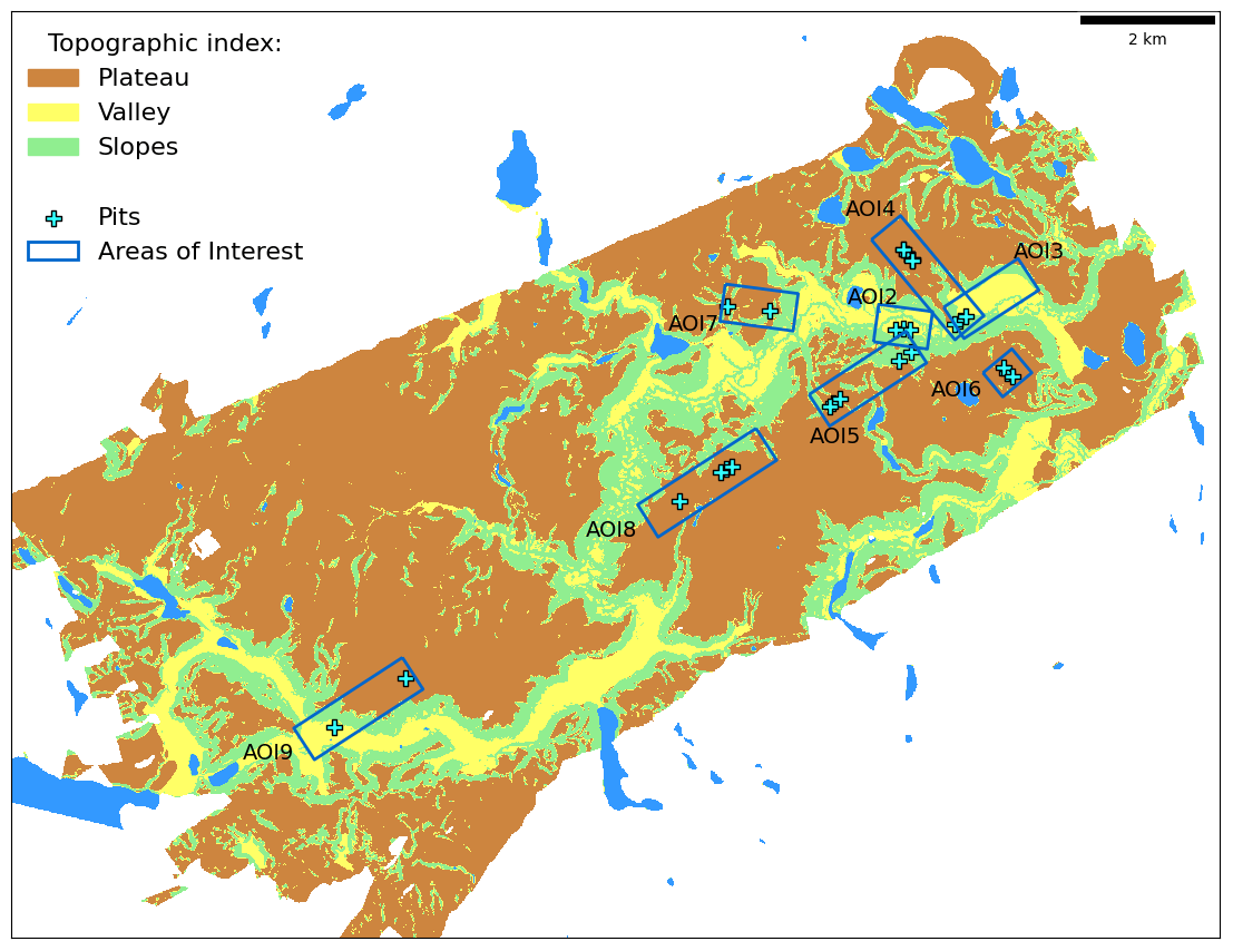
Figure 1 Topographic index of Trail Valley Creek, Northwest Territories (NWT), Canada, with locations of snow pits and areas of interest for airborne data. Adapted from Rutter et al. (2019).

2 Methods

2.1 Ground data

Ground-based measurements of snow microstructure and microwave emission were made throughout the catchment of TVC, NWT, Canada (68°44^′17^′′ N, 133°26^′26^′′ W), between 14 and 22 March 2018. The elevation range is 9 to 187 m a.s.l. and the topography is mostly gently rolling slopes with some deep valleys (Marsh et al., 2010). The dominant land surface is tussocks (37 %), followed by dwarf shrubs (24 %), whereas trees only constitute 2 %. Further details about the vegetation characteristics are available in Grünberg et al. (2020). Figure 1 shows how the catchment was topographically divided into areas of flat upland plateau (<5° ground slope), flat valley bottom (<5°) and slopes (>5°) (Rutter et al., 2019) and highlights areas of interest (AOIs) selected for study prior to the field measurements. Further contextual information about seasonal changes in TVC and drone-based structure-from-motion snow depth measurements within the AOIs is available in Walker et al. (2021), with some differences in AOI numbering and dimensions from this study. Snow pit measurement locations (Fig. 1) were selected in order to capture a wide range of topographies, aspects and vegetation characteristics of TVC, which are also representative of the wider Arctic tundra in general. In addition, snow pit locations were linearly aligned along three flight lines to allow spatially coincident comparisons of airborne measurements with measured and simulated microwave emissions from the surface.

Vertical profiles of snow properties (density, specific surface area (SSA), temperature and stratigraphy) required to simulate microwave scattering in snow were measured in 29 snow pits. In each pit, density, SSA and temperature were measured at a 3 cm vertical resolution. Densities were measured using a 100 cm³ gravimetric cutter and SSA was measured using two measurement systems, an InfraRed Integrating Sphere (IRIS) (Montpetit et al., 2012) and an A2 Photonic Sensors IceCube, both of which followed the method of Gallet et al. (2009) using infrared reflectance of snow samples at 1310 nm in an integrating sphere. For density and SSA, the average of two replicate samples at each position in the vertical profile was taken in the majority of snow pits in order to account for horizontal heterogeneity across the snow pit wall. Snowpack layers (including ice lenses) were identified through visual inspection and hardness tests and classified according to Fierz et al. (2009). Additionally, following Rutter et al. (2019), snow layers were grouped into one of three microstructure types, i.e. surface snow (SS), wind slab (WS) or depth hoar (DH), through comparative assessment of all profile measurements in combination with each other, as shown in Fig. 2. The majority of snow pits were between 20 and 40 cm deep. Pits 6-3W and 18-5W were located in drifts, leading to depths closer to 1 m. Depth hoar was present in all the pits. Pit 5-3E did not have a wind slab layer, and only a thin wind slab layer was present in pit 4-3C1. Several pits did not have a fresh surface snow layer present. Almost all the pits had an ice crust present, with the exception of pit 24-8C.

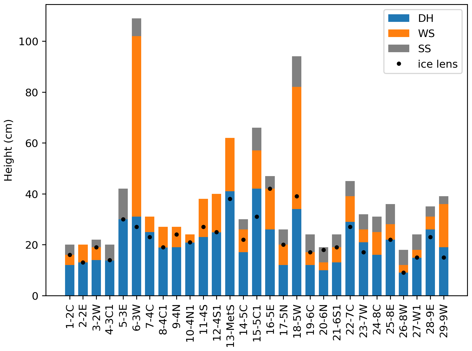
Figure 2 Stratigraphy of individual snow pits within areas of interest. Depth hoar (DH) layers are shown in blue, wind slab (WS) layers are shown in orange and surface snow (SS) layers are shown in grey. The locations of ice lenses are shown with the black dots.

At 10 pit locations, coincident measurements of passive microwave TBs at 89 GHz, in both vertical and horizontal polarizations, were made by a surface-based radiometer (Langlois, 2015). The radiometer was mounted on a sled at a height of approximately 1.5 m above and at an angle nadir to near-horizontal snow surfaces. A 6 dB beam width of 3° meant the measurement footprint on the snow surface was approximately 0.15 m × 0.15 m. Radiometers were calibrated using ambient (blackbody) and cold (liquid nitrogen) targets and had a worst-case measurement error of 2 K based on six ambient blackbody calibration checks made during the campaign. At each location, TB measurements were made over a 6 s integration time for a minimum of 3 min. Mean TBs were calculated and the standard deviation used as a quality control flag. Three measurements were made at each site and the radiometer was moved by 2.5 m between each measurement. Coincident physical temperatures were made at the base and within the snowpack.

2.2 Airborne data

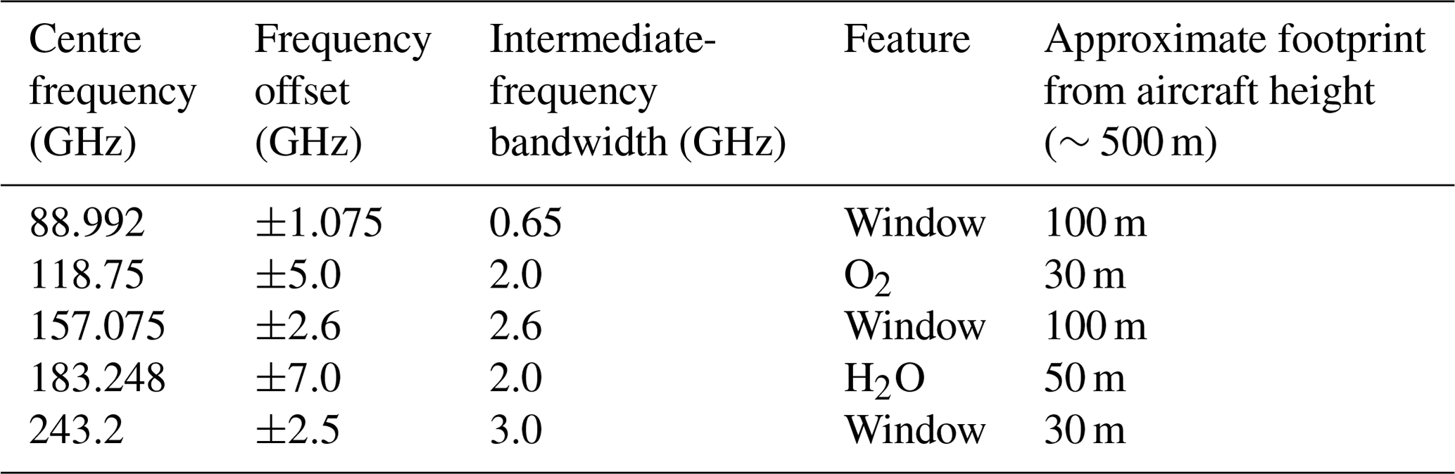
During MACSSIMIZE, the Facility for Airborne Atmospheric Measurements (FAAM) BAe-146 atmospheric research aircraft was based in Fairbanks, Alaska. Five flights were flown over TVC and followed a series of low-level (approximately 500 m altitude) flight lines that aligned with the snow pits. This paper focuses on data for two flights, C087 and C090, on 16 and 20 March 2018, as these flights were free of low cloud and occurred within the same period as ground observations were made. Airborne measurements were made using the Microwave Airborne Radiometer Scanning System (MARSS; McGrath and Hewison, 2001) and the International Submillimetre Airborne Radiometer (ISMAR; Fox et al., 2017) on board the FAAM aircraft. Both instruments are along-track scanning radiometers containing dual-sideband heterodyne receivers measuring between 89 and 664 GHz. This paper concentrates on channels up to 243 GHz as frequencies higher than this will not have significant sensitivity to the surface except in very dry environments due to strong water vapour absorption. A summary of the channels used in this study is given in Table 1. Processing of MARSS and ISMAR data produces Rayleigh–Jeans-equivalent TBs (Fox et al., 2017).

The radiometers are mounted on the side of the aircraft, allowing both upward and downward views, and contain a rotating scan mirror with a fully configurable scan pattern. A typical scan cycle rotates through multiple upward and downward scene views, plus views of two calibration targets (one ambient and one heated). During MACSSIMIZE, the instruments remained at a single downward-viewing angle when over the AOIs, with calibration and zenith views in between, to increase the number of observations made over the surface sites. Downwelling sky observations at multiple angles are shown in Appendix A1. This paper uses observations where the instruments pointed in a near-vertical nadir direction (±5°) when over the AOIs, which occurred during C087 and two runs of C090. Most of the MARSS and ISMAR receivers detect a single linear polarization (of the channels studied in this paper, only the 243 GHz window channel offers dual orthogonal polarization), with the polarization angle depending on the instrument scan angle. This must be considered for non-nadir observations; however, in this paper only near-vertical nadir observations are used, where the impact of polarization angles is minimal.

Table 1 MARSS and ISMAR channel definitions for the frequencies used in this study.

2.3 SMRT modelling

The SMRT model was previously described in Picard et al. (2018). Briefly, this is a multi-layer snow scattering model suitable for passive, active and radar altimeter applications (Larue et al., 2021). It has a modular structure that allows different modelling configurations, including an electromagnetic model and a radiative transfer solver. For the simulations presented in this paper, the Improved Born Approximation (IBA) electromagnetic model and the DORT radiative transfer solver were used to simulate brightness temperatures emitted from the surface of the snowpack, given the snowpack properties described later in this section. SMRT was coupled with ARTS to account for the atmospheric emission and absorption necessary at these higher frequencies and to simulate TB at the height of the aircraft. Results presented in this paper use nadir, vertically polarized TB to evaluate SMRT against ground-based and airborne observations. Atmospheric adjustment of the ground-based radiometric data to the height of the aircraft for comparison with airborne data is described later in Sect. 2.4.

“Base” SMRT simulations describe default parameterizations and neglect within-layer measurement variability or other potential sources of error considered later in this study. These base simulations were constructed from the three-layer dataset described in Sect. 2.1 and shown in Fig. 2. Observations of layer thickness, temperature and density were used directly to create SMRT layers. However, SMRT requires microstructure model parameters rather than the SSA observed in the field. To link with previous studies (Harlow and Essery, 2012; King et al., 2018; Vargel et al., 2020), an exponential microstructure model was chosen for this study. SSA was used to derive the required exponential correlation length with the modified Debye relationship (Mätzler, 2002; Montpetit et al., 2012):

$$\begin{array}{}\text{(1)}& l_{\mathrm{ex}}={\mathit{\alpha }}_{\mathrm{db}}{\displaystyle \frac{\mathrm{4}(\mathrm{1}-\mathit{\rho }/{\mathit{\rho }}_{\mathrm{i}})}{\text{SSA}{\mathit{\rho }}_{\mathrm{i}}}},\end{array}$$

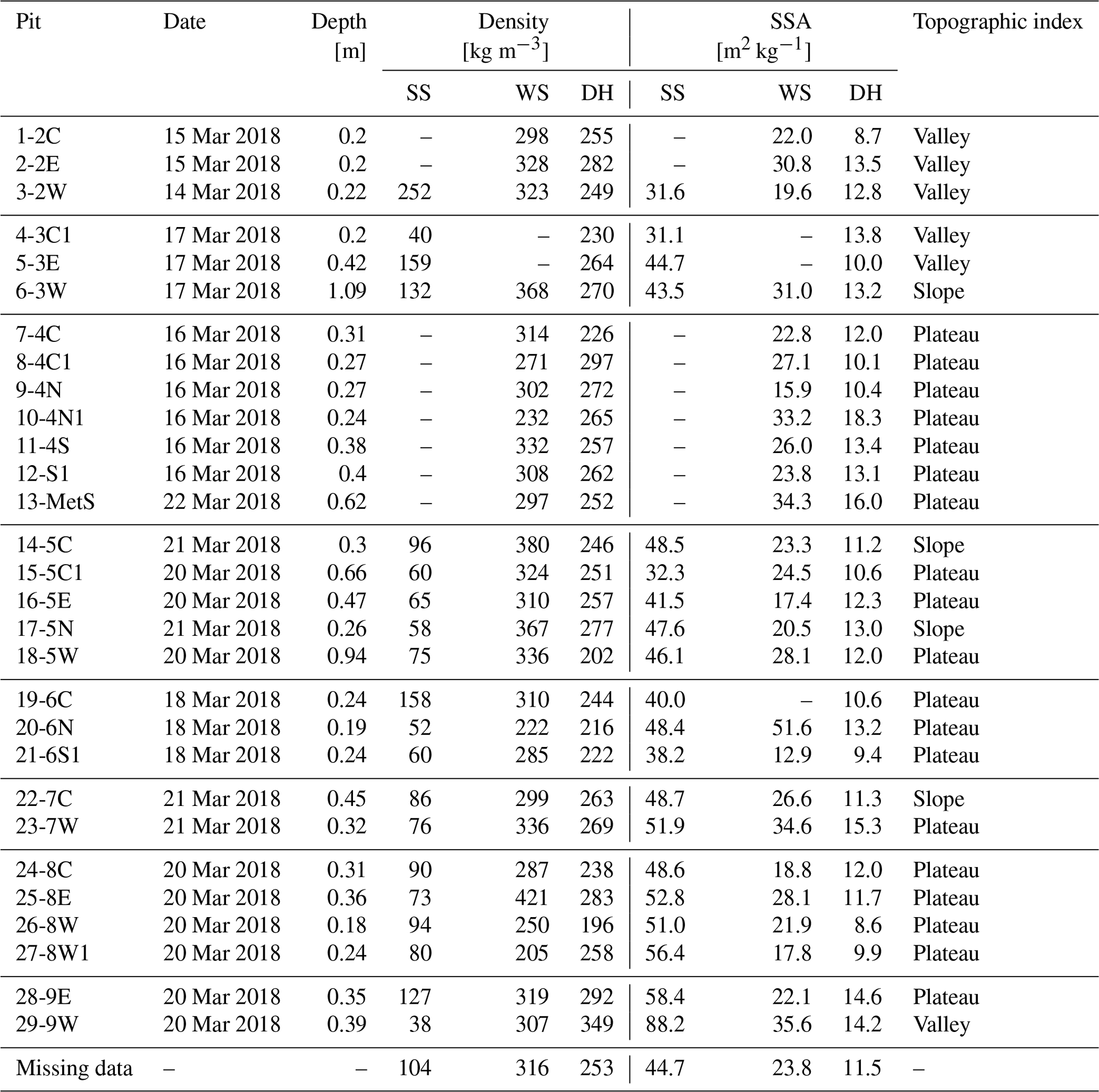
where the Debye modification parameter α_db is assumed to be 0.75 for surface snow and wind slab layers (Mätzler, 2002) and 1.2 for depth hoar (Leinss et al., 2020) in the base simulations, ρ is the snow density and ρ_i is the density of pure ice. The value of α_db=1.2 for depth hoar was chosen after initial assessment of the modelling strategy through a sensitivity study described below. For snow pits with dual density and SSA observation profiles, the mean layer values between profiles were used in the base simulations. Table 2 illustrates the density and SSA values used for each pit and the values taken from Rutter et al. (2019) used for missing observation values in layers that were too thin. The underlying soil surface is assumed to be flat, with a temperature of 258.15 K and a permittivity of 4−0.5j based on the work of King et al. (2018) at TVC. As snow pit observations were made over an 8 d period under varying atmospheric conditions, SMRT snow layer temperatures were linearly interpolated from the air temperature at the time of the flights to the mean of the measured temperatures (263 K) in the lowest snow layer on flight days.

Table 2 Snow pit properties used for base SMRT simulations. Snow pit numbering is sequential, followed by the AOI (2–9) and the location within the AOI (north, east, south, west or central). Density and specific surface area (SSA) are given for the surface snow (SS), wind slab (WS) and depth hoar (DH) layers. In layers that were too thin to measure, properties were gap-filled from the “Missing data” values taken from Rutter et al. (2019). Flight overpass data used in this paper were from 16 and 20 March 2018.

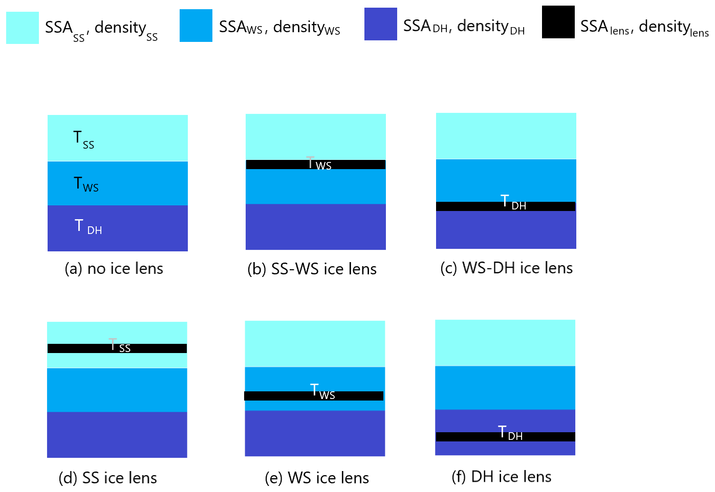
An ice lens was present in almost all the snow pits but occurred at different locations within the layers as shown in Fig. 2. Coherent effects of ice lenses have not been implemented in SMRT, but dielectric contrast boundary effects of ice lenses are taken into account in this study. Where ice lenses were present, an additional layer was inserted into the snowpack. The recorded height of the ice lens was used to inform the strategy for amending the layering structure of the snow. As illustrated in Fig. 3, for an ice lens at the boundary between layers, the thickness of the lower layer is reduced in order to maintain the correct total snow depth and the ice lens inserted, leading to a four-layer snowpack. If the ice lens occurs within a layer, then that layer is split, with the thickness of the top section given by the height of the top of the layer minus the height of the top of the ice lens. The thickness of the lower section is recalculated to maintain the total snow depth. This results in a five-layer snowpack to represent an ice lens embedded within one of the three original layers. The ice lens density is assumed to be 909 kg m⁻³ (Watts et al., 2016) and the SSA is assumed to be 100 m² kg⁻¹ (extremely weakly scattering, mainly boundary effects), with the ice lens thickness given by the field measurements. The measured ice lens thickness ranged from 1 mm to 1 cm, with a mean of 2 mm.

Figure 3 Modelling strategy to account for ice lenses in the three-layer snowpack.

Uncertainty associated with the simulation approach was assessed using pit 9-4N as a case study at 89 GHz. At this frequency, simulations are expected to be more sensitive to processes lower in the snowpack than at other frequencies. Phenomena observed in some pits but not accounted for in the base simulations include air gaps at the snow–soil interface and formation of surface crusts. There is also variability in observed depth, SSA and density. Finally, the modified Debye parameter α_db is not known but is often taken as 0.75 from Mätzler (2002). Leinss et al. (2020) indicated that this value may be as high as 1.2 for depth hoar, which is within the range found by Vargel et al. (2020), who considered variability in this parameter with frequency and snow type. Here, for simplicity, we compare the case where all layers have α_db=0.75 with the case where the depth hoar layer has α_db=1.2.

The sensitivity of simulated TBs to modelling assumptions is shown in Table 3. A basal air gap was included by inserting a 5 mm layer of low-density (10 kg m⁻³) snow and an exponential correlation length of 10 µm. This, however, had a negligible effect on the TB, as did incorporating a depth observation uncertainty of 2 cm (applied to the depth hoar layer thickness). Including a surface crust of thickness 5 mm with the ice lens density and an exponential correlation length of 10 µm lowered the TB by 4.5 K. A more realistic Debye modification of 1.2 applied to only the depth hoar layer resulted in a larger drop in the TB of 5.7 K. This impact cannot be ignored and demonstrates a potential deficiency in the use of the “standard” Debye correction factor of 0.75. However, the largest impact on the TB was found by representing the layer density and SSA using the largest and smallest observed values within each layer of each pit. Including all effects resulted in a TB range of 164–193 K, close to the full range of AOI4 airborne observations from the C087 flight over areas within AOI4 classified as plateau, which was 163–201 K (see Table 3).

Table 3 Sensitivity results for snow pit 9-4N, used to define modelling protocol based on a comparison with airborne observations at 89 GHz over plateau regions of AOI4. The effect of the flight C087 atmosphere (see Sect. 2.4) is included.

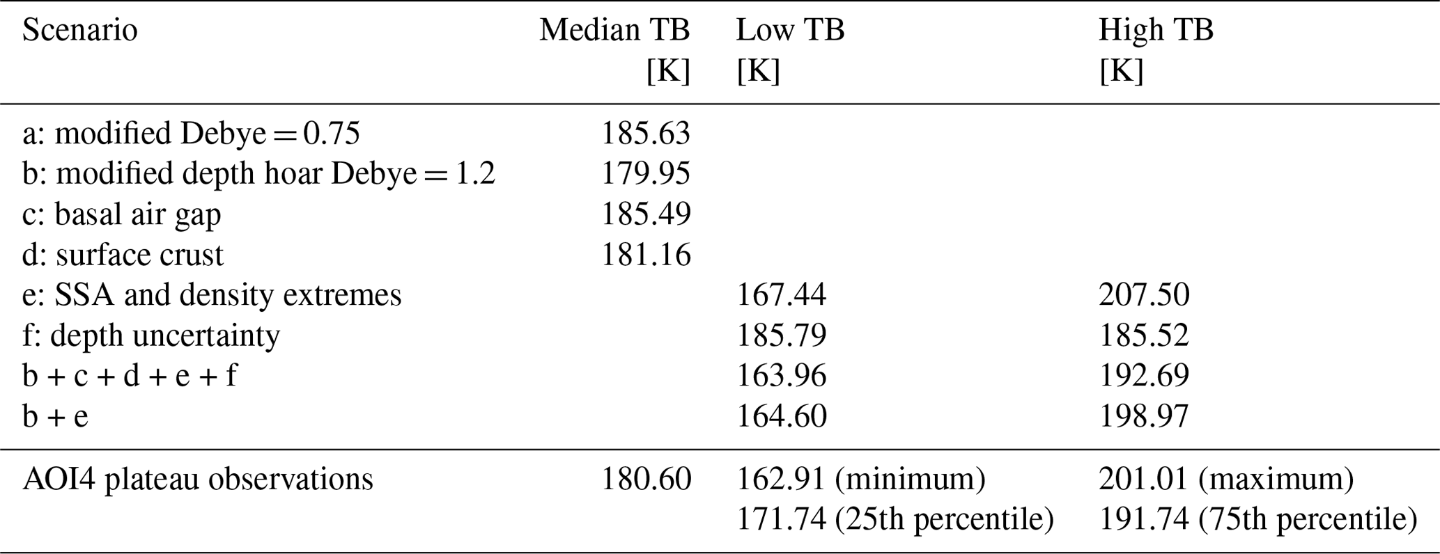
All simulations presented in the “Results” section use the new Debye modification of 1.2 for the depth hoar layer (0.75 for all other layers). Surface crusts are neglected due to the difficulty in determining whether they are present or not, but they could be a source of error. Basal air gaps and uncertainty in depth are neglected due to the lack of sensitivity to them. “Base case” simulations are driven by the median in microstructural properties, but the minimum and maximum measurements of SSA and density are also used to determine variability in simulations. When including atmospheric effects, this leads to a simulated TB range of 165–199 K for pit 9-4N (scenario b + e in Table 3), which is comparable with the airborne observations.

2.4 Adjusting for the atmosphere

For this paper, the ARTS (Eriksson et al., 2011; Buehler et al., 2018) has been used to simulate the angle-dependent atmospheric radiation for SMRT. The ARTS Clear Sky (non-scattering) solver is used for a 1D atmosphere. The sensor is represented using a “top-hat” channel response in each of the two sidebands, with a frequency resolution of 0.1 GHz. The simulated atmosphere accounts for the atmospheric downwelling contribution to the surface signal (radiation transmitted into the snowpack and radiation reflected by the surface) that distinguishes simulations for each flight day, and it is used to adjust for the layer of the atmosphere between the aircraft and the surface when comparing airborne observations with surface-based radiometer observations and simulations. Surface TBs were adjusted to aircraft height using

$$\begin{array}{}\text{(2)}& T_{\mathrm{b},\mathrm{adj}(\mathit{\theta },\mathit{\nu })}={\text{Tr}}_{(\mathit{\theta },\mathit{\nu })}{T}_{\mathrm{b},\mathrm{s}(\mathit{\theta },\mathit{\nu })}+T_{\mathrm{b},\mathrm{up}(\mathit{\theta },\mathit{\nu })},\end{array}$$

where T_b,adj is the adjusted surface TB at angle θ and frequency ν, Tr is the atmospheric transmission which determines the attenuation of the surface signal, T_b,s is the unadjusted surface TB (which includes downwelling atmospheric radiation scattered by the snow) and T_b,up is the upwelling TB due to atmospheric emission. A flowchart illustrating the loose coupling between SMRT and ARTS and their processing steps is given in Appendix A2.

The atmospheric impact is expected to be greatest for the atmospheric sounding channels due to absorption and emission by oxygen (118 GHz) and water vapour (183 GHz). However, the atmospheric window channels (89, 157 and 243 GHz) also have some sensitivity to the atmosphere due to the water vapour continuum and far wings of water vapour and oxygen absorption lines. In this paper, the channels furthest from the centre of the atmospheric absorption lines at 118 and 183 GHz were chosen because strong oxygen and water vapour absorptions at the channels closer to the absorption line centres mean there is little sensitivity to the surface, and these channels would be less useful for verifying SMRT.

Temperature and water vapour profiles used as input for ARTS were retrieved for each AOI on each flight. Background profiles were taken from a combination of dropsonde profiles, sondes released before the low-level AOI runs and profiles from the Met Office operational global NWP model (above sonde height). The retrieval adjusts these background profiles to match aircraft-level downwelling observations in the vicinity of each AOI at 183±1, ±3 and ±7 GHz. Because downwelling observations are only available above the aircraft, the profile below the aircraft height is not adjusted in the retrieval. The height at the bottom of each profile is determined by interpolating to the mean ground height of the AOIs. Due to the instruments remaining at nadir over the AOIs, downwelling observation data in the full range of zenith viewing angles have been taken for periods of 30 s either side of the AOI overpass.

Within ARTS, water vapour absorption is calculated using the AER v3.6 line parameters with the MT_CKD v3.2 continuum. Oxygen absorption is calculated using the Tretyakov et al. (2005) model. Simulated downwelling TBs using the ARTS absorption model configuration mentioned here are compared with observations in Appendix A1 for the full range of zenith viewing angles. The figure in Appendix A1 demonstrates how atmospheric downwelling varies with viewing angle and therefore why it is important to represent the anisotropy of the atmospheric radiance.

SMRT and therefore the ARTS configuration used return thermodynamic TBs. As stated in Sect. 2.4, MARSS and ISMAR processing produces Rayleigh–Jeans-equivalent TBs, and therefore SMRT simulations are converted to a Rayleigh–Jeans equivalent before comparison with airborne observations by applying a frequency-dependent offset given by $h\mathit{\nu }/\mathrm{2}k$, where h is Planck's constant, ν is frequency and k is Boltzmann's constant. A discussion of the different TB definitions and the derivation of the offset can be found in Han and Westwater (2000).

3 Results

3.1 SMRT evaluation against ground data

Figure 4 compares SMRT TB at 89 GHz with nadir ground-based TBs measured by the sled-mounted radiometers. SMRT simulations are the mean of the two flights and are then adjusted to ground level with the inversion of Eq. (2). The range of simulations captures the observations, with the exception of pits 21-6S1 (plateau pit) and 4-3C1 (valley pit). The low TB simulated in 4-3C1 is later attributed to a very low surface density, whereas low wind slab SSA drives the discrepancy in 21-6S1 (see Sect. 3.2). The base simulations (shown with blue circles) tend to overestimate high TB and underestimate low TB. Overall, the mean difference is −7.1 K and the root mean squared difference is 16.6 K. Removal of outliers 4-3C1, 20-6N and 21-6S1 reduces the mean difference to −0.03 K and the root mean squared difference to 7.5 K. This is quantified in terms of a difference rather than an error, as measurements themselves may be subject to small distortions due to shadowing of the sky and emission from the radiometers.

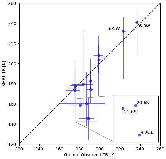
Figure 4 Comparison between SMRT simulations and ground-based radiometer observations at 89 GHz (nadir). Blue circles show the mean of ground observations and TB simulation using mean measured snow properties and blue lines show the range of the ground observations and the TB simulation range using combinations of maximum and minimum measured SSA and density. The zoom box is used to provide space to label these specific pits.

Ground-based radiometer observations are adjusted to the height of the aircraft and compared with airborne observations in Fig. 5. Airborne observations include all those within the AOI and over the same topography classification as the pit, with the central point showing the median value and error bars indicating the inter-quartile range. Most observations are grouped but have larger variability in the ground-based observations. Pits 6-3W (slope) and 18-5W (plateau) had a much higher TB observed on the ground than from the aircraft. These pits had the deepest snow, as shown in Fig. 2, and were located in drifts. Figure 5 illustrates the challenges in using airborne data to evaluate ground-based point simulations, given that the footprint may be different in size and location.

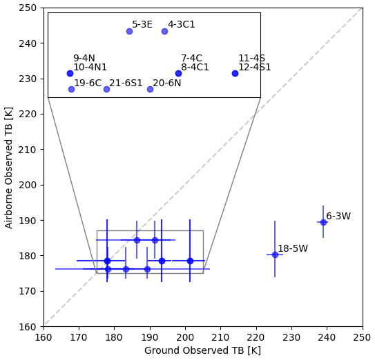
Figure 5 Comparison between ground-based observations of brightness temperature and airborne brightness temperature at 89 GHz for pits where observations were available. Airborne observations from both C087 and C090 flights were used and ground-based observations have been adjusted to the height of the aircraft. Blue circles show the mean of ground observations and the median of airborne observations and blue lines show the range of ground observations and the inter-quartile range of airborne observations. The zoom box is used to provide space to label all the pits. Note that pits 7–12 are paired pits within close proximity to its pair.

Differences in ground and airborne footprint locations are shown in Fig. 6, where data from the C087 flight have been plotted according to their calculated ground coordinates. Some areas of interest have pits (shown with crosses) relatively close to the line of flight, e.g. AOI7 and AOI9, whereas others, e.g. AOI5, AOI6 and AOI8, have a line of pits parallel to the flight data. TBs along the airborne transects appear to show a topographic signal: plateau areas tend to have low TB and sloped or transition areas high TB. This is shown clearly for AOI7 in Fig. 6 but is evident in other areas of interest. Some transects contain TB signatures not easily identifiable from the topographic map (e.g. high TB in the north-east of AOI8), but this could be due to smaller-scale heterogeneity in the underlying surface, the snow properties or the vegetation. Given the difference in footprint location, it is plausible that selection of the closest airborne TB may not be representative of TB at pit locations as the underlying topography may be very different. Because of the difficulties in matching a given snow pit location with a representative airborne footprint, for comparison with SMRT simulations, all airborne observations over a particular topography class (plateau, slope, valley) were grouped within each AOI. In this way, valley pit simulations were compared with all the valley airborne observations within its AOI, and likewise for the pits located on slopes and plateaus.

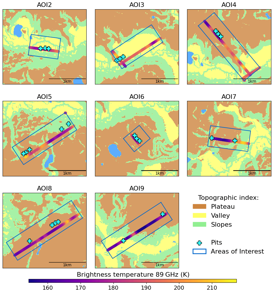
Figure 6 Variation in airborne brightness temperature observed on flight C087 in each area of interest. Snow pit locations are indicated with crosses.

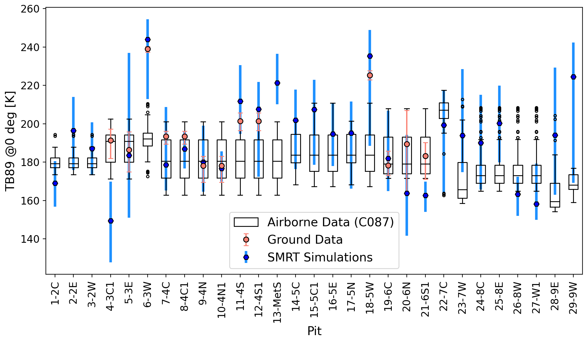
Figure 7 Comparison between SMRT simulations of microwave brightness temperature at 89 GHz, V polarization, near-nadir incidence angle, ground-based measurements and flight C087 airborne observations from the MACSSIMIZE field campaign. SMRT and ground-based TBs have been adjusted to the height of the aircraft. Airborne data: box (inter-quartile range), horizontal black line (median), vertical black lines (whiskers extending from the end of each box to 1.5 times the inter-quartile range) and black circles (outliers beyond this range). Ground data: filled orange circle (mean) and vertical orange line (range). SMRT simulations: filled blue hexagon (TB using mean measured snow properties) and vertical blue line (TB range using combinations of maximum and minimum measured SSA and density).

3.2 SMRT evaluation against airborne data

Figure 7 compares the simulated TB from each of the 29 pits with the airborne observations within the same AOI and topographical index. Simulated TB at 29 pits overlapped the airborne TB range in all but four pits, which are examined in further detail later in this section. SMRT had good agreement with ground-based TB at 6-3W but not at 4-3C1 or 21-6S1, which is consistent with Fig. 4. Ground-based TB was not available for the Met station snow pit. Analysis of pits grouped by their underlying topography (see Table 2) provides a test of how well SMRT simulations are able to explain the observed broad-scale spatial variability in TB.

Valley pits in AOI2 are simulated well, with overlap between simulations and observations. The western (3-2W) base simulation (blue hexagon) lies within the airborne whiskers. Variability in microstructure parameters in the eastern and central pits 2-2E and 1-2C leads to a larger range in simulated TB that overlaps the median of airborne TB, demonstrating that SMRT can be used to represent airborne TB adequately. Other valley pits (5-3E, 29-9W and 4-3C1) also have a large range in simulated TB.

There is close agreement between airborne median TB, ground TB and the SMRT base simulation despite the large variation in microstructure at valley pit 5-3E. SMRT underestimates TB at valley pit 4-3C1. Table 2 indicates that pit 4-3C1 also had an unusually low surface density. If the “Missing data” value from Table 2 is used in the base simulation instead of the low surface density, TB increases from 149.3 to 156.2 K and is therefore much closer to the observations.

Four snow pits were dug in areas classified as sloped topography. These were 6-3W, 14-5C, 17-5N and 22-7C. At 6-3W, SMRT simulations are higher than and outside the range of airborne observations. There is, however, close agreement with ground TB measurements, indicating that the airborne observations may not have observed the drift containing 6-3W. The remaining slope pits show good agreement with airborne observations, with 14-5C SMRT simulations covering the inter-quartile range of the airborne observations and 17-5N and 22-7C simulations covering the extent of the whiskers. For pit 22-7C, the simulations also capture the few low TB outliers.

Plateau pits are generally simulated well, with the exception of the Met station and 21-6S1. Simulated TB at the Met station is too high compared with airborne observations, which indicates an underestimation of scattering. The Met station is situated in AOI4, along with three sets of paired pits. Observations 7-4C and 8-4C1 were made in adjacent pits, and the ground-based radiometric observations made at pit 8-4C1 were assumed to be representative of 7-4C. Similarly, the radiometric observations at 10-4N1 and 12-4S1 were assumed to be representative of 9-4N and 11-4S. The agreement between ground observations and the SMRT base case is better for the pits where the radiometric observations were made, i.e. 8-4C1, 10-4N1 and 12-4S1. These adjacent pits in AOI4 give insight into the simulated microwave behaviour relative to the input data. At the central site, simulated TB is lower at 7-4C than at 8-4C1, which is consistent with the deeper snowpack and larger WS grains at 7-4C. The northern site is really interesting. TB at 9-4N is higher than at 10-4N1 despite a smaller SSA (almost half that of 10-4N1 in both the WS and DH layers). This is in contrast to the expectation that a smaller SSA means larger grains, more scattering and lower TB.

The Met station's pit was the only pit dug later than flights C087 and C090 and after a strong wind event (discussed later in this section) that redistributed snow, so simulations may not be representative of the airborne observations made beforehand. However, analysis of post-wind event flight data shows similar results to the C087 and C090 flights, suggesting that this may not be the cause of the discrepancy. SSA observed at the Met station was generally high, as shown in Table 2, but it was similar to that of pit 10-4N1. With Table 2, “Missing data” SSA values were applied to all the layers and the base TB decreased from 221.3 to 213.0 K. Conversely, pit 21-6S1 TB simulations are too low compared with both airborne and ground-based TB observations, which indicates too much scattering. Table 2 shows very low SSA for the WS layer (large grains) and values that would be more representative of depth hoar. If default “Missing data” values were used for the SSA values in all the layers, TB would increase from 162.6 to 172.1 K, which would be closer to the observations.

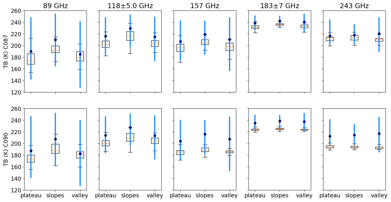
Figure 8 Boxplot comparison between SMRT simulation (including atmosphere, adjusted to aircraft height) and airborne observations at 89, 118, 157, 183 and 243 GHz grouped by topographic type. Results for the C087 flight are shown on the top and results for the C090 flight are shown on the bottom. Airborne data: box (inter-quartile range), horizontal orange line (median) and vertical black lines (whiskers extending from the end of each box to 1.5 times the inter-quartile range). SMRT simulations: filled blue hexagon (TB using mean measured snow properties) and vertical blue line (TB range using combinations of maximum and minimum measured SSA and density).

Figure 8 compares SMRT simulations with observations at frequencies between 89 and 243 GHz for the two flights (C087 and C090) over all the snow pits, grouped by topographic type. TB range and sensitivity of observed TB to topography decrease with increasing frequency, indicating less dependence on surface properties. Observed TB variability generally decreases from flight C087 to flight C090, as shown by changes in the inter-quartile range in Fig. 8. Between the flights there is little change in the median TB for 89 and 118 GHz, but there is a decrease at 157 GHz and above. SMRT simulations differ little between the flights (only the atmospheric contribution changes in the simulations), leading to less overlap between simulations and observations at 183 and 243 GHz for flight C090.

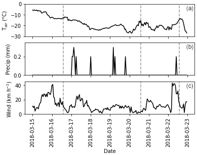
Figure 9 Hourly meteorological data from the Trail Valley Creek station for the duration of the MACSSIMIZE campaign. (a) Air temperature (°C), (b) precipitation (mm) and (c) wind speed (km h⁻¹). Dashed lines indicate flight timings: C087 on 16 March, C090 on 20 March and C092 on 22 March 2018. Data from Government of Canada (2024), station WMO ID 71683.

Surface snowpack structure at the time of snow pit measurement may differ from the surface structure at the time of the flights. Figure 9 shows precipitation events and changes in air temperature and wind speed throughout the field campaign. Timings of three flights are also shown with dashed vertical lines. No significant changes are expected in layer microstructure throughout the course of the field campaign, as the temperature remained below freezing and only small changes in SSA can be expected over the days between the flights. However, after flight C087 on 16 March there were several snowfall events. Snow pit data from 4-3C1 on 17 March (Table 2) indicate that the surface snow had an unusually low density of 40 kg m⁻³. Most snow pits after 17 March had surface snow densities of less than 100 kg m⁻³. Air temperature decreased after flight C087, with a cold spell between flights C087 and C090. Wind speed was relatively low between flights C087 and C090, but there was a period of high wind speeds (maximum 43 km h⁻¹) between flight C090 on 20 March and flight C092 on 22 March, which led to observed redistribution of surface snow after the blizzard, mostly removing snow above the ice lens in flat areas.

To examine the potential impact of surface change on TB and to investigate whether this can account for the differences in the observed TB between flights in Fig. 8, a thin, fresh surface snow layer was added to all the snow pits. The additional surface snow layer was assumed to have similar properties to the surface layer of pit 4-3C1, i.e. a thickness of 5 cm, a density of 40 kg m⁻³, a temperature of 260 K and an exponential correlation length of 0.1 mm. The difference in TB is shown for each frequency in Table 4 and is shown in Fig. A3. Additional surface snow decreases the brightness temperatures at all the frequencies. The absolute difference is small (<2.2 K) at 89 and 118 GHz, moderate at 183 GHz (2.1–3.5 K) and larger at 157 and 243 GHz (6.2–14.4 K). Given that the penetration depth decreases with frequency, it could be expected that the effect of the surface layer should increase with frequency, but this is not the case for 183 GHz, where the effect is smaller than at 157 GHz. This suggests that emission from the atmosphere itself may dominate over the impact of the additional surface snow layer at 183 GHz, which is consistent with the higher measured and simulated emission at 183 GHz shown in Fig. A1.

Table 4 Effect of a thin surface snow layer on simulated median brightness temperatures for different topographical land surface types (K). Brightness temperature difference is calculated for snow pits with 4-3C1 surface snow minus snow pits as measured. Negative values indicate that inclusion of low-density surface snow reduces the brightness temperature.

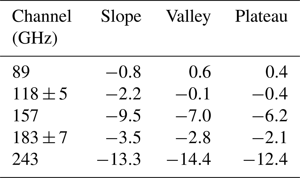
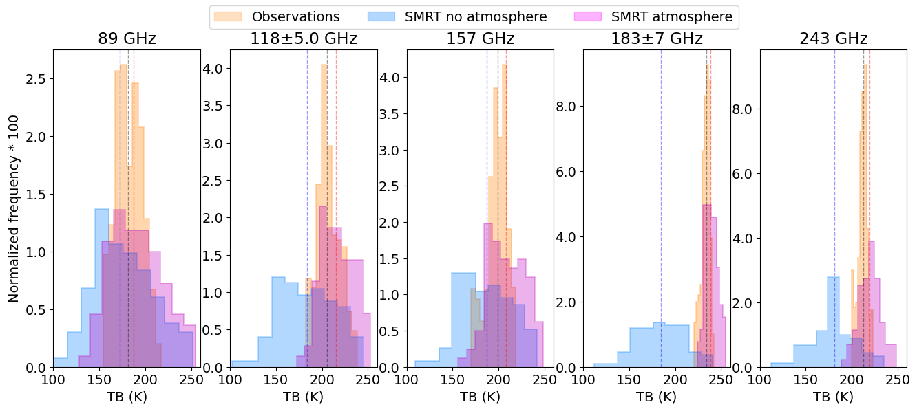
Figure 10 Histogram of brightness temperatures for all frequencies showing the impact of neglecting atmospheric contribution in SMRT simulations. Observations are for flight C087 only, aggregated over AOI and topographical surface type. Dashed lines show distribution medians: black for observations, blue for SMRT with no atmosphere and red for SMRT simulations incorporating atmospheric effects.

The importance of including the atmosphere at different frequencies is demonstrated in Fig. 10. Overall, inclusion of the atmosphere reduces the root mean squared difference (RMSD) of the base simulation medians by frequency and flight from 23 to 14 K. At an individual pit level, comparison with airborne data of the same topography classification (i.e. plateaus, slopes or valleys) reveals that inclusion of the atmosphere reduces the RMSD from 35.7 to 18.4 K with the atmosphere included for flight C087 (n=145). For flight C090 the RMSD without the atmosphere is 29.2 K, and with the atmosphere it is 21.7 K. The impact of the atmosphere is largest at 183 GHz and smallest at 89 GHz. Inclusion of the atmosphere narrows the range of simulated TB. Atmospheric emission increases simulated TB, as shown by the shift in the median (from blue to red dashed lines in Fig. 10) despite atmospheric attenuation of emitted radiation from the snow surface. For all frequencies, the median TB including the atmosphere is closer to the observations than simulations without the atmosphere. However, Kolmogorov–Smirnov two-sample tests of distribution equivalence show that simulated distributions (either with or without the atmosphere) are statistically different to distributions of airborne observations at a 5 % significance level.

4 Discussion

The aim of this study was to evaluate whether SMRT could be used to explain observed microwave behaviour at frequencies needed to improve numerical weather prediction in the Arctic. With anisotropic atmospheric radiance modelled with ARTS, SMRT captures the distinction between snow overlying different topographies. The frequency dependence is also simulated well. The good agreement here supports the applicability of IBA electromagnetic theory at higher frequencies. With an estimated limit of wavenumber $k_{\mathrm{0}}\sim \mathrm{1.5}\times$ radius of spheres to keep the error of the approximation within reasonable limits, as specified by Picard et al. (2022), the IBA upper frequency limit for the largest scattering depth hoar layer in Table 2, i.e. 8.6 m² kg⁻¹, is around 188 GHz. Inclusion of the atmosphere reduces the simulated RMSD to a value that could be expected from comparisons with ground-based observations at frequencies more sensitive to snow. An RMSD of 14 K for the base simulations here is within the range of 13–26 K reported in the literature in the frequency range 19–89 GHz (Roy et al., 2016; Royer et al., 2017; Vargel et al., 2020) given similar in situ microstructure data.

Underlying topography is relevant at 89 GHz but becomes less relevant at higher frequencies. As frequency increases, penetration depth decreases and a sensor may only see the upper portion of the snowpack. This is the dominant effect and results in smaller differentiation between TB classified by ground topography. However, structural changes and spatial variability in snowpack properties driven by topography may result in a topographical signal in the TB despite the signal not penetrating to the base of the snowpack. Small differences between topographical types persist even at 243 GHz in Fig. 8.

Variability in ground observations of microstructure led to large variation in simulated TB and good overlap with airborne observations for the majority of the snow pits. This demonstrates the value of making multiple measurements within the snowpack as the simulations cover a range of plausible TBs at a point given the best available snowpack structure information. Kolmogorov–Smirnov tests show that the simulations and airborne observations have different distributions, even with the atmosphere taken into account. This may be expected as airborne observations capture more of the terrain than individual pits, which were chosen to maximize variability rather than provide random statistical sampling of the region (which would not be feasible given the number of pits required to do so). There is the issue of scale, as the simulations use point measurements, whereas the airborne footprint covers an area of up to ∼100 m in diameter. Whilst snow pit simulations should lie within the range of airborne simulations and for the most part do, it is possible that the differences in ground footprint location mean that snow conditions in the snow pits were not sampled along the aircraft transects. In some cases there are clear differences in location (Fig. 6), and pits 6-3W and 18-5W were located in drifts not captured in the airborne transect. The spatial extent of the drift is also smaller than the airborne footprint, so even if the flight transect had completed a direct overpass, the drift contribution to airborne observations may be limited. Further improvements could be gained with a better understanding of how to relate pit measurements to larger-scale microstructure variability. This may be possible with rapid measurement instruments such as the snow micropenetrometer in conjunction with local pit calibration as demonstrated by King et al. (2020) and Dutch et al. (2022).

It is vital to know the relative thicknesses of layers, as these can override microstructural differences by changing the penetration into lower, larger-grain-sized layers. This is demonstrated by the paired pits 9-4N and 10-4N1, where 9-4N TB was higher than 10-4N1 TB despite smaller SSA (i.e. larger grains, more scattering) in the 9-4N snow pit layers. The difference here is driven by the thinner WS layer in 10-4N1. More of the signal is proportionally affected by the DH grains than for 9-4N, leading to lower TB. The importance of the relative thickness of the depth hoar layer has already been highlighted in other studies (King et al., 2018; Rutter et al., 2019; Meloche et al., 2022) and is consistent with the higher sensitivity of surface layer changes at 94 GHz compared with the lower frequencies found by Wiesmann et al. (2000).

Identification of low-precipitation events with deposition of low-density, small-grain-sized surface snow will be important for use of these data in NWP. Although atmospheric conditions differ between the 2 flight days, the differences are too small to explain the low TB observed by flight C090. A change in microstructure rather than a change in atmospheric conditions may explain the difference in the observed TB. Meteorological and in situ data presented here suggest deposition of low-density snow between the first two flights that was then removed, redistributed or heavily compacted by wind between the second and third flights, leading to similar observed TB for the first and third flights but lower TB for the second flight. Smooth-surface ice lenses facilitated wind redistribution and removal of the surface snow. Addition of thin, low-density, fresh surface snow in the simulations supports the hypothesis that the difference in observed TB is driven by snow microstructural differences between flights. In the simulations, the mass of snow added is small and the exponential correlation length is also small, which means that the scattering within that layer is small. The difference in brightness temperature is likely due to the high (density-driven) dielectric contrast between layers caused by the unusual low-density fresh snow. The effect is largest at 243 GHz, where the penetration depth is shallowest. The difference at 183 GHz could be expected to exceed that at 157 GHz because of the shallower penetration depth at the higher frequency. It does not because the effect of the atmosphere is larger at 183 GHz.

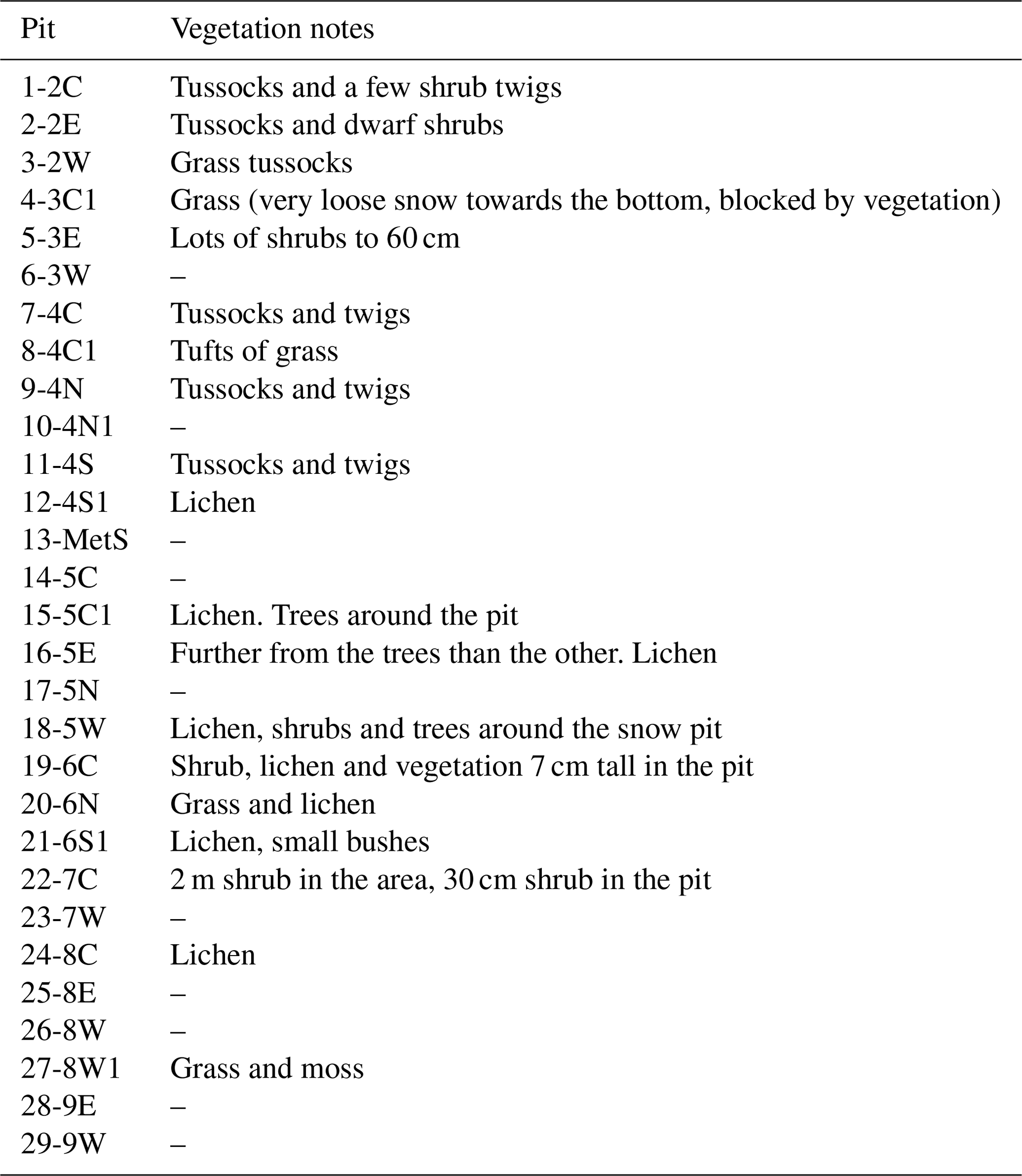
The demonstrated ability of SMRT to represent TB variability over different snow-covered topographies in TVC indicates the potential value of using SMRT to improve atmospheric retrievals given snowpack information. Vegetation may have contributed to modelling error as this was noted in many pits (see Table A1) but was not taken into account in modelling, and this has yet to be implemented in SMRT. However, in pits with lots of vegetation noted (shrubs of up to 60 cm in pit 5-3E and 30 cm shrub in pit 22-7C), SMRT base simulations are within 1.5 times the inter-quartile range of airborne observations. Although contributions from twigs and grasses are likely to be small, the change in snow structure due to vegetation in pit 4-3C1 (very loose snow towards the bottom and blocked by vegetation) could be a contributing factor to the discrepancy between observations and simulations. It is difficult to sample snow density and SSA within vegetation, and shrubs alter the snowpack properties, increasing depth hoar (Royer et al., 2021). In general, there is good overlap with observations, with some differences between simulated TB and airborne measurements that can be explained by local variability in microstructure, changing meteorological conditions, differences in measurement location and/or footprint size.

In current numerical weather prediction models, microwave emissivity is assumed to be constant over snow-covered surfaces, is derived from a monthly climatology or is retrieved dynamically with emissivity assumed to be constant over frequency (Di Tomaso et al., 2013; Geer et al., 2014). However, in some channels, errors in these approaches are too large to be able to use satellite observations in the Arctic. Instead, SMRT could be used to parameterize the surface radiometric behaviour. This would require good microstructure, layer thicknesses and identification of surface snow from the NWP land surface model. Optimizing assimilation of satellite observations has been identified as the most effective way of improving forecast skill in the Arctic (Laroche and Poan, 2022). NWP systems already use radiative transfer models but require higher-accuracy models for snow (e.g. the vertical polarization bias at 89 GHz is currently $\sim -\mathrm{35}$ K: Hirahara et al., 2020, Fig. 13). This should be possible with SMRT. Alternative approaches with dynamic emissivity depending on frequency can also be supported through SMRT modelling.

This modelling study encompassed dry snow conditions only, but wet snow conditions must also be considered in future work for operational numerical weather prediction models. Although the emissivity and temperature of uniformly wet snow are well-known, within-footprint spatial distribution of melt is important for simulation of brightness temperatures (e.g. Vuyovich et al., 2017). The ability of land surface models to capture spatial and temporal variability in wet snow, especially freeze–thaw cycles, is important if these data are to be used to their full capacity in numerical weather prediction. Future work will focus on how we can use SMRT to quantify observation uncertainty from satellite measurements at microwave frequencies over snow-covered regions and consequently how to use the atmospheric information within them to improve weather forecasts in the Arctic.

5 Conclusions

In this study, SMRT was evaluated at frequencies between 89 and 243 GHz in an Arctic tundra snow environment with dry snowpacks, with the atmospheric contribution estimated with ARTS. It was found that there was good agreement between simulations and airborne observations despite differences in footprint location and size. At 243 GHz, the electromagnetic model used is potentially outside the range of applicability, but the good agreement may be partly because the larger grain sizes start to approach the wavelength of radiation located deeper in the pack and therefore contribute less to the signal as the penetration depth decreases. Inclusion of the atmospheric emission and scattering, such as with ARTS, is essential for accurate simulation and interpretation of ground-based, airborne and satellite observations of microwave emission in surface-sensitive atmosphere channels.

Here, a clear topography-related signal was evident at the lower frequencies, but the distinction between sloped, valley and plateau areas diminished as frequency increased. This is because the penetration depth of radiation decreases with frequency and, at higher frequencies, less of the signal comes from the lower portion of the snowpack. Differences between adjacent snowpacks demonstrated that, in addition to microstructure, accurate knowledge of layer thickness is critical for determining whether the deeper snow layers are seen by the sensors. The ability of snowpack models to simulate these parameters is an important area of research, particularly for land surface models used in numerical weather prediction systems.

Spatial variation in brightness temperatures observed with airborne instruments is reflected by the simulations, which indicates potential for use of SMRT to interpret satellite observations needed for numerical weather prediction. Meteorological events, i.e. the addition of fresh, low-density precipitation and a later wind event that removed it over the space of a few days, likely caused differences in observed brightness temperatures. The effects of this event were largest at 157 and 243 GHz as the signal is more weighted to the surface of the snow but is somewhat dampened by the atmospheric contribution at 183 GHz. This study has shown how snow microstructural and stratigraphic information can have different influences depending on the frequency of the observations used. A strategy to account for spatial and temporal variability in snow microstructure is much needed for future implementation in numerical weather prediction systems and for use of Arctic microwave satellite observations in weather forecasts.

Appendix A: Supplementary material

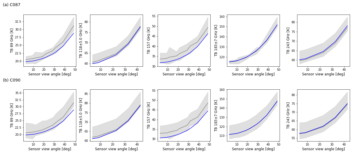
Figure A1 Simulated (blue) vs. observed mean and range (grey) downwelling brightness temperatures in the full range of zenith viewing angles, averaged across the AOIs at 89, 118±5.0, 157, 183±7 and 243 GHz for flights C087 (a) and C090 (b).

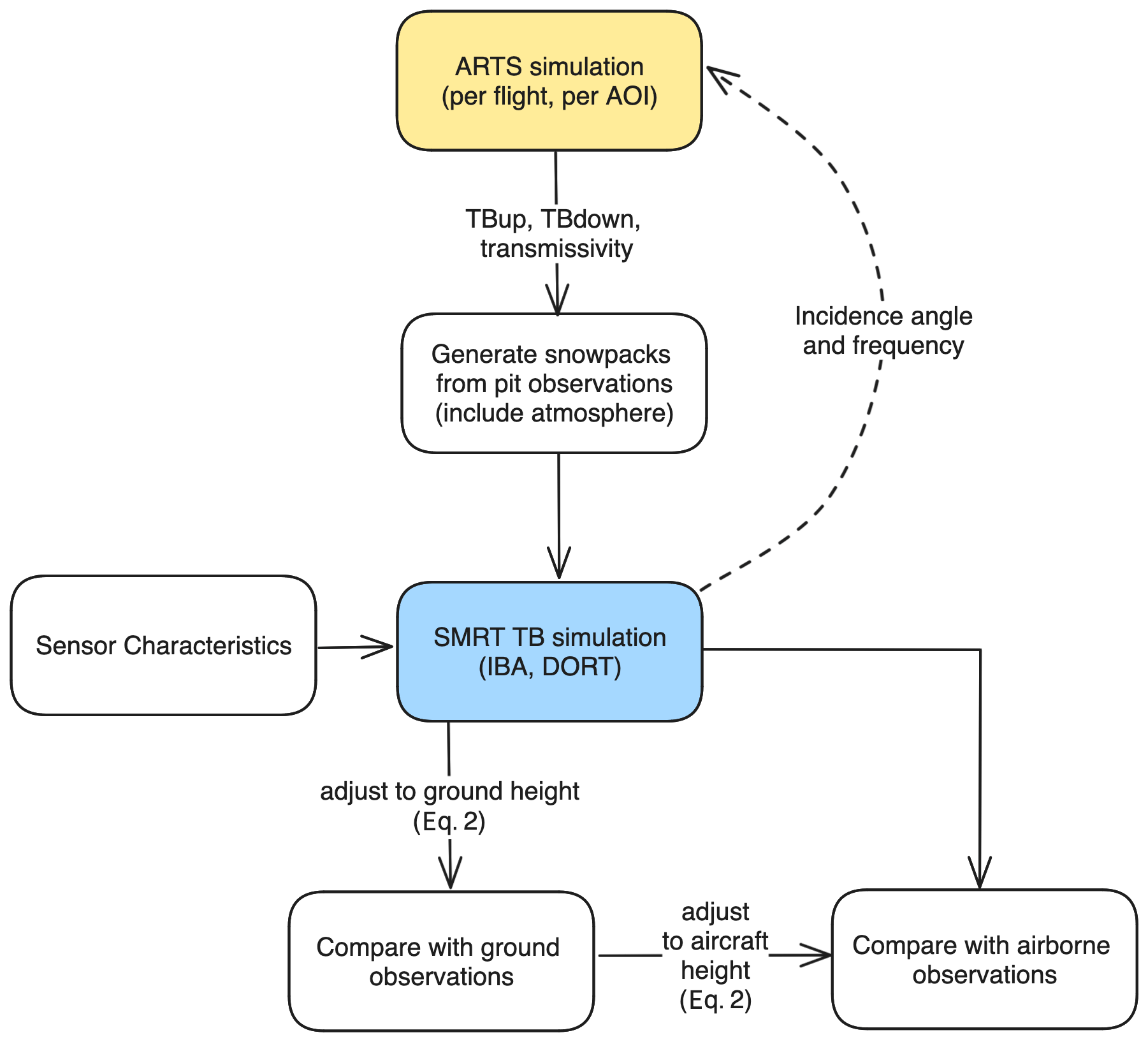
Figure A2 Flowchart demonstrating SMRT–ARTS coupling and processing steps for comparison with observations. ARTS atmospheric properties are used to calculate upwelling TB (TBup), downwelling TB (TBdown) and atmospheric transmissivity matrices used in the SMRT snowpacks. Although ARTS is configured as an initial step under the assumption of a surface blackbody, calculation of the atmospheric properties is carried out dynamically during the SMRT simulation as the matrices depend on the array of incidence angles and the frequencies of the sensors. Equation (2) is used to adjust SMRT simulations to surface height for comparison with ground-based sensors (Fig. 4) and for adjustment of ground observations to account for the atmosphere beneath the aircraft (Figs. 5 and 7).

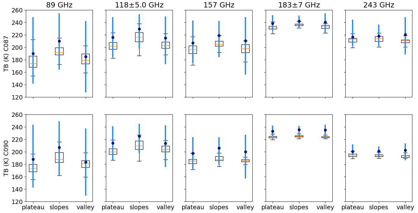
Figure A3 Boxplot comparison between SMRT simulation (including atmosphere, adjusted to aircraft height) and airborne observations at 89, 118, 157, 183 and 243 GHz grouped by topographic type. Results for the C087 flight are shown on the top and results for the C090 flight are shown on the bottom. A thin surface snow layer has been added for flight C090 simulations. Airborne data: box (inter-quartile range), horizontal orange line (median) and vertical black lines (whiskers extending from the end of each box to 1.5 times the inter-quartile range). SMRT simulations: filled blue hexagon (TB using mean measured snow properties) and vertical blue line (TB range using combinations of maximum and minimum measured SSA and density).

Table A1 Vegetation at each pit as recorded in field notes.