Misidentified subglacial lake beneath the Devon Ice Cap, Canadian Arctic: a new interpretation from seismic and electromagnetic data

In 2018 the first subglacial lake in the Canadian Arctic was proposed to exist beneath the Devon Ice Cap, based on the analysis of airborne radar data. Here, we report a new interpretation of the subglacial material beneath the Devon Ice Cap, supported by data acquired from multiple surface-based geophysical methods in 2022. The geophysical data recorded included 9 km of active-source seismic-reflection profiles, seven transient electromagnetic (TEM) soundings, and 17 magnetotellurics (MT) stations. These surface-based geophysical datasets were collected above the inferred locations of the subglacial lakes and show no evidence for the presence of subglacial water. The acoustic impedance of the subglacial material, estimated from the seismic data, is 9.49 ± 1.92 × 10⁶ kg m⁻² s⁻¹, comparable to consolidated or frozen sediment. The resistivity models obtained by inversion of both the TEM and MT measurements show the presence of highly resistive rock layers (1000–100 000 Ω m) directly beneath the ice. Re-evaluation of the airborne reflectivity data shows that the radar attenuation rates were likely overestimated, leading to an overestimation of the basal reflectivity in the original radar studies. Here, we derive new radar attenuation rates using the temperature- and chemistry-dependent Arrhenius equation, and when applied to correct the returned bed power, the bed power does not meet the basal reflectivity threshold expected over subglacial water. Thus, the radar interpretation is now consistent with the seismic and electromagnetic observations of dry or frozen, non-conductive basal material.

1 Introduction

Analysis of radio echo sounding (RES) data acquired in 2011–2015 (Rutishauser et al., 2018) and 2018 (Rutishauser et al., 2022) proposed that the first subglacial lake in the Canadian Arctic had been detected beneath the Devon Ice Cap (DIC) (Fig. 1a). The proposed lake covered an area of 11.6 km² and was identified from a combination of higher relative basal RES reflectivity (proxy for dielectric contrast between two materials) and specularity content (proxy for wavelength-scale roughness) over a hydraulically flat region (Rutishauser et al., 2018, 2022). These are characteristics that are consistent with the typical signature of subglacial lakes (e.g. Carter et al., 2007). The proposed lake was located in a trough beneath 760 m of ice near the summit of DIC ($\mathrm{75}\mathit{°}{\mathrm{19}}^{\prime }{\mathrm{2.26}}^{\prime \prime }$ N, $\mathrm{82}\mathit{°}{\mathrm{46}}^{\prime }{\mathrm{32.62}}^{\prime \prime }$ W), in a region where the ice was thought to be frozen to the bed (Van Wychen et al., 2017). Recent temperature modelling suggested cold basal temperatures estimated between −10 and −14 °C (Rutishauser et al., 2018). Therefore, without surface meltwater input, the inferred subglacial lake beneath DIC required a high salinity content to depress the freezing point and enable water to exist in its liquid form at the estimated cold basal temperatures. Thus, the lake was proposed to be hypersaline (Rutishauser et al., 2018), where geologic modelling suggested that the solute for the brine came from an underlying evaporite-rich sediment unit containing interbedded salt sequences, called the Bay Fiord Formation (Rutishauser et al., 2018).

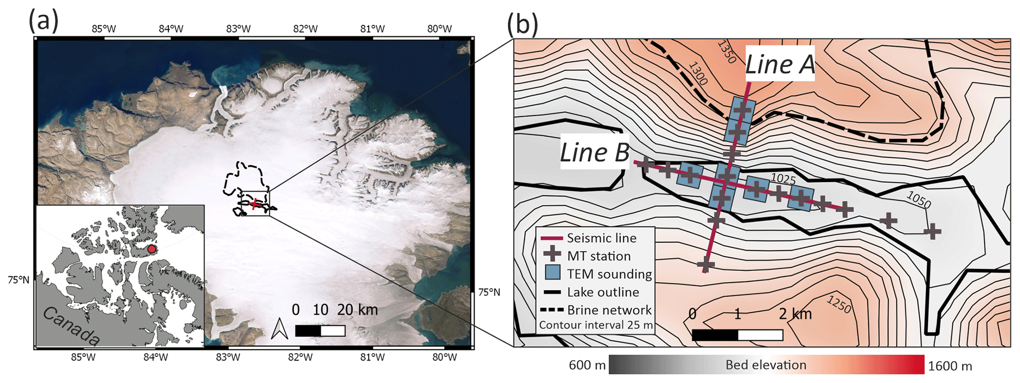
Figure 1 (a) Regional map of DIC (ESRI satellite world imagery) with subglacial lake, T2 (black line), and brine network (dashed black line) proposed from RES (Rutishauser et al., 2018, 2022). (b) Enlarged area shows the bed elevation measured from RES with seismic, TEM, and MT survey locations.

RES data are highly effective at mapping the ice–base boundary and have excellent spatial coverage. However, as with all geophysical methods, multiple interpretations can fit a RES dataset. For example, anomalously strong and continuous basal reflections in RES data could indicate the presence of (1) subglacial water (Carter et al., 2007), (2) water-saturated and highly conductive sediment (Tulaczyk and Foley, 2020), or (3) smooth bedrock/sediments (Hofstede et al., 2023; Jordan et al., 2017). Furthermore, water usually contains significant dissolved salts and is electrically conductive. This results in significant attenuation of radar signals through the skin-depth effect. This means that reflections from structures at the bottom of lakes are rarely observed in RES data, making it difficult to distinguish a subglacial lake from a layer of saturated sediments or a thin sheet of water at the glacier bed. Finally, difficulties in constraining radar attenuation rates can lead to misinterpretation of basal conditions (Matsuoka, 2011). The non-uniqueness of RES interpretations can be overcome with complementary geophysical surveys, such as active-source seismic and electromagnetic (EM) methods. Seismic, EM, and radar data are sensitive to different material properties of the subsurface, and the combination of the three methods offers more robust evidence of subglacial water.

Seismic methods provide acoustic properties of the ice–base interface, which can give independent material properties of the subsurface to confirm the presence of a subglacial lake. The acoustic impedance (product of density and compressional wave velocity) contrast across the ice–base interface provides information on whether the material directly under the ice is acoustically soft (e.g. a lake, negative polarity reflection) or acoustically hard (e.g. consolidated sediment, positive polarity reflection) relative to ice. Seismic methods are also capable of measuring lake depth since water is not attenuated to seismic energy. Therefore, where available, seismic evidence is key for diagnosing the presence and thickness of a subglacial lake.

EM techniques, such as transient electromagnetics (TEM) and magnetotellurics (MT), measure the subglacial electrical resistivity structure and are particularly applicable for glacial hydrological studies due to the large difference in electrical resistivity between ice (10 000–100 000 000 Ω m) and water (0.1–100 Ω m) (Key and Siegfried, 2017). Furthermore, the electrical resistivity of water decreases rapidly with salinity (Killingbeck et al., 2021). However, EM methods are sensitive to the conductance, the product of conductivity (inverse of electrical resistivity) and thickness, rather than the layer resistivity or thickness alone. Therefore, a thinner, more conductive layer (e.g. thin hypersaline lake) can produce a similar EM signal to a thicker, less conductive layer (e.g. thick package of saturated sediments), making it difficult to determine the exact layer thickness and resistivity. By integrating multiple geophysical techniques with different resolution capabilities, for example, RES, seismic, and EM, layer thicknesses can be accurately constrained, allowing for a reliable determination of the subsurface resistivity structure (Killingbeck et al., 2021).

The RES-inferred presence of a subglacial lake beneath DIC motivated a new campaign of multi-technique ground-based geophysical surveys in 2022 to examine the properties of the hypothesized lake, to characterize the lake complex, and thereafter to sample the subglacial water. Here, active-source seismic, TEM, and MT data were collected in the same field campaign. The joint acquisition of TEM and MT methods to characterize a subglacial lake is a novel approach. The data were recorded on two profiles and included 9 km of active-source seismic-reflection data, 7 TEM soundings, and 17 MT stations. One profile was acquired across the location of the proposed lake, extending into a region where a brine network was believed to be present (line A; Fig. 1b). A second profile was acquired along the long axis of the proposed lake (line B; Fig. 1b). In this study, we present the results from the seismic and electromagnetic data acquired over the inferred subglacial lake, which leads to a new interpretation of the subglacial material beneath DIC. Using the new data and interpretation, we reanalysed the RES data presented in Rutishauser et al. (2018, 2022). This leads to a different interpretation of the RES reflectivity data which is now consistent with the seismic and electromagnetic observations presented in this study.

2 Geophysical methods

2.1 Active-source seismic reflection

2.1.1 Acquisition and processing

The active-source seismic-reflection data acquisition consisted of a moving spread of 48 vertical component geophones of 40 Hz spaced 10 m apart along two profiles (A and B; Fig. 1). For each spread, we collected data at 11 shot locations using an 8 kg sledgehammer impacting a thick steel plate. At each source location, at least five hammer shots were stacked into a single shot gather to increase the signal to noise ratio. The shot locations for each spread were at offsets −60, 0, 120, 240, 360, 480, 530, 590, 650, 710, and 770 m from the first geophone. After data were collected at each of the 11 shot locations, the spread was moved 470 m along the survey line, and the data collection was repeated. For line A, the seismic line was moved a total of 9 times, obtaining reflection points at the ice–base interface spaced every 5 m along a 4500 m distance. For line B, the seismic line was moved a total of 10 times, obtaining reflection points at the ice–base interface spaced every 5 m along a 5000 m distance. The in-line resolution of the migrated data and the vertical resolution is 9 m (assuming one-quarter wavelength, λ). In theory, water layers down to $\mathit{\lambda }/\mathrm{32}$ (1 m) can be detected; however, amplitudes from these layers may not be representative of their elastic properties due to seismic tuning (Booth et al., 2012).

Seismic processing was completed using MATLAB and the open-source CREWES package available from http://www.crewes.org (last access: 4 July 2022). The processing steps included the following:

1. apply shot-to-shot energy variation correction along the line (method follows that applied in King et al., 2008);

2. remove bad traces;

3. perform bandpass filtering (80, 90, 250, 260 Hz);

4. perform bandpass filtering in the FK domain (−0.025, −0.035, 0.025, 0.035);

5. mute airwave using a velocity of 333 m s⁻¹;

6. apply a top mute;

7. apply FK fan filter between 500 and 5000 m s⁻¹;

8. apply NMO correction using a velocity of 3700 m s⁻¹ and DMO correction using a velocity of 3902 m s⁻¹ over the steeply dipping valley side (where the dip angle is estimated at 18.510 from the bed DEM);

9. stack the data;

10. apply post-stack finite-difference migration using a velocity of 3700 m s⁻¹.

2.1.2 Normal incident reflection method

The strength of the reflection from the ice–base interface (R1) can indicate its acoustic properties and, hence, allow for the determination of the material that is likely present, i.e. water or rock. To estimate the acoustic properties of the ice–bed interface (R1), we first calculate the reflection coefficient by analysing the amplitudes of R1 and its multiple. The basal reflection coefficient c_R can be determined as a function of incidence angle θ using

$$\begin{array}{}\text{(1)}& c_{\mathrm{R}}\left(\mathit{\theta }\right)=\mathrm{2}{\displaystyle \frac{A_{\mathrm{M}\mathrm{1}\left(\mathit{\theta }\right)}}{A_{\mathrm{R}\mathrm{1}\left(\mathit{\theta }\right)}}}{e}^{aL\left(\mathit{\theta }\right)},\end{array}$$

where A_R1 and A_M1 represent the amplitude of the first and second (the multiple) ice bottom reflections, respectively; a is the absorption coefficient; and L is the ray path length of the R1 reflection. We use the multiple bounce method (Maguire et al., 2021; Horgan et al., 2021) and the normal incidence approximation where only traces with an incident angle < 10° were used. Here, our hammer and plate impulse source has a minimum-phase source signature. Therefore, our data are at the minimum phase (as we have not applied deconvolution to zero-phase our data during the seismic processing); hence, the reflections are represented by a minimum-phase wavelet. We picked the absolute maximum energy of wavelets R1 and M1 by defining a window around the minimum-phase wavelet. We assumed an attenuation a=0.27 km⁻¹ (Horgan et al., 2012). This attenuation corresponds to a seismic-quality factor (Q) of 30–300 for 10–100 Hz waves in a 3860 m s⁻¹ medium. We estimate c_R in the trough to be 0.468 ± 0.116. c_R can then be used to determine the acoustic impedance (Z_b) of R1 using

$$\begin{array}{}\text{(2)}& Z_b=Z_{\mathrm{ice}}{\displaystyle \frac{\mathrm{1}+c_{\mathrm{R}}}{\mathrm{1}-c_{\mathrm{R}}}},\end{array}$$

where Z_ice is ∼ 3.33 × 10⁶ kg m⁻² s⁻¹.

2.2 Electromagnetics

2.2.1 Transient electromagnetics

TEM data were acquired with a Geonics PROTEM67 system consisting of a three-channel digital time-domain receiver unit, a vertical component multi-turn receiver coil (area 100 m²), and a TEM67 generator-powered transmitter. A 500 m × 500 m square transmitter loop was set out using snow mobiles and PVC stakes at each of the four corners, with 3.3 Ω km⁻¹ resistance wire. The receiver coil was placed 250 m outside of the loop, 250 m away from the generator-powered transmitter module. The transmitter loop locations are shown in Fig. 1. Background noise levels, measured with the transmitter coil turned off, are considered low at DIC since there are no large sources of electrical noise, e.g. power lines, buildings, roads, and metal infrastructure. Background noise readings were acquired with noise level at 2 × 10–11 V m⁻². At each location the transmitter module was used to power 23 A of current around the large loop (500 m × 500 m). Base frequencies of 7.5 and 3 Hz were acquired with 30 measurement time gates, 120 s integration time, and 10 stacks, meaning each sounding took 1 h and 30 min. The time–amplitude decay curves measured during each sounding (Fig. B1 Appendix B) were inverted to obtain a 1D resistivity profile with depth (Killingbeck et al., 2020).

In Fig. B1, the negative received voltages recorded at the early time gates (< 0.1 ms) are likely due to an oversaturation from remanent current still in the transmitter loop, after the turn-off time, when the receiver measurement period begins. We removed these negative data and any adjacent positive data which look to be distorted (flatten) from the oversaturation (0.1–0.2 ms). At the late times (> 3 ms), we observe a flip from positive to negative data, highlighting that there is an induced polarization (IP) effect on our data and the likely existence of chargeable material in the subsurface (Weidelt, 1982). The observation of an IP effect on our TEM data suggests a high-resistivity subsurface (e.g. Grombacher et al., 2021), where the resistive background heightens the IP response from the Earth, contrary to the existence of a conductive hypersaline lake.

Here, we invert the positive TEM data for a normal decay curve to give an indication of the resistivity range of the ice and subglacial material. We use the open-source MATLAB code MuLTI-TEM (Killingbeck et al., 2020) to invert the data using a trans-dimensional Bayesian inversion method that determines the posterior probability density function of resistivity as a function of depth (Killingbeck et al., 2020). The Bayesian inversion method will always choose a simple model (e.g. thick layers with small resistivity changes) unless constrained by additional geophysical data. Here, the inversion is constrained by ice thicknesses at each sounding location, derived from RES data (Rutishauser et al., 2022), where the resistivity bounds are limited between 1000 and 1 000 000 Ω m in the ice layer. At depths below the ice, the resistivity bounds are set between 0.1 and 1 000 000 Ω m. The inversion parameters used in MuLTI-TEM are shown in Appendix B in Tables B1 and B2.

2.2.2 Magnetotellurics

MT uses natural electromagnetic signals to image the subsurface resistivity structure. In MT exploration, the depth of investigation increases as the frequency decreases; thus, frequency can be considered a proxy for depth. Data were recorded with Phoenix Geophysics MTU-5C instruments. Electric fields were measured with 100 m long dipoles connected to the ice with titanium sheet electrodes and custom high-impedance amplifiers. Magnetic fields were measured with Phoenix Geophysics MTC80H induction coils that were buried in the snow. The station deployment is shown in Fig. 1. Line A had seven stations with 500 m spacing and was orthogonal to the trend of the trough that was inferred to contain a subglacial lake. Line B had 10 stations and was parallel to the trend of the trough. At each station MT time series data were recorded for 24–48 h at sample rates of 24 000 Hz and 150 Hz. The stations were deployed in a geographic coordinate system because it was not possible to use a compass owing to the high magnetic inclination.

The time series data were processed using a statistically robust algorithm of Egbert (1997). This produced high-quality estimates of apparent resistivity, phase, and tipper in the frequency band 100–0.01 Hz. The dimensionality of the DIC MT data were investigated using the phase tensor approach (Caldwell et al., 2004). The phase tensor gives a graphical representation of how the measured MT data vary with the azimuth of the coordinate system used to plot the data. This analysis of dimensionality of the data is required to determine which inversion approach (1D, 2D or 3D) is most suitable for the data.

• If the subsurface has a 1D resistivity structure, then the phase tensor will plot as a circle and the skew angle will be zero.

• A 2D resistivity structure will result in elliptical phase tensors, also with zero skew angle. The strike direction will be aligned with either the major axis or the minor axis of the ellipse.

• A 3D structure will result in an elliptical phase tensor and a non-zero skew angle. By looking at the phase tensors as a function of frequency, information can be obtained about the depth variation of the resistivity structure.

Thereafter, a 2D inversion was implemented using the code of Rodi and Mackie (2001). The starting model was generated in the WinGLink software package and included the ice layer with the base elevation taken from recent RES data (Rutishauser et al., 2022). The ice was assigned a resistivity of 100 000 Ω m (estimated from the results of the TEM Bayesian inversion; Fig. 6) and fixed in the inversion. Furthermore, a tear (discontinuity in resistivity) was allowed at the base of the ice to avoid excessive smoothing. This tear enables a sharp contrast in resistivity between the ice and subglacial material directly beneath the ice in the inversion model, if required to fit the data observations. Furthermore, a number of 2D inversions were run to allow for the optimal degree of smoothing, known as the trade-off parameter (τ; Rodi and Mackie, 2001), to be determined. Here, a value of τ=3.2 was chosen as it defines the corner of the trade-off curve representing an optimum balance for fitting the measured MT data without obtaining an unrealistically rough model (Fig. C1 in Appendix C).

2.3 Deriving RES attenuation rates

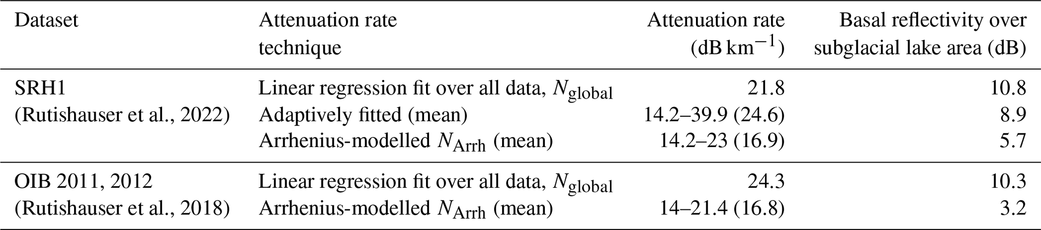
To calculate basal reflectivity, the radar energy loss through dielectric absorption of the overlying ice (englacial attenuation rates) must be estimated. Attenuation rates are commonly derived directly from RES data via linear regression fits between the observed bed power and ice thickness (Rutishauser et al., 2018, 2022; Gades et al., 2000; Schroeder et al., 2016a, b). However, attenuation rates can also be predicted from a temperature- and chemistry-dependent Arrhenius equation (MacGregor et al., 2007, 2015). At DIC, the linear regression fit method from the previous studies provided attenuation rate estimates of 21.8 dB km⁻¹ (regression fit over the entire dataset; Rutishauser et al., 2022) and 26.8 dB km⁻¹ (mean of a regression fit on a profile-by-profile basis; Rutishauser et al., 2018), yielding a relatively high basal reflectivity that was interpreted as a subglacial lake. However, considering the new seismic, TEM, and MT results, we hypothesize that these attenuation rates were overestimated, leading to an overestimation of the basal reflectivity.

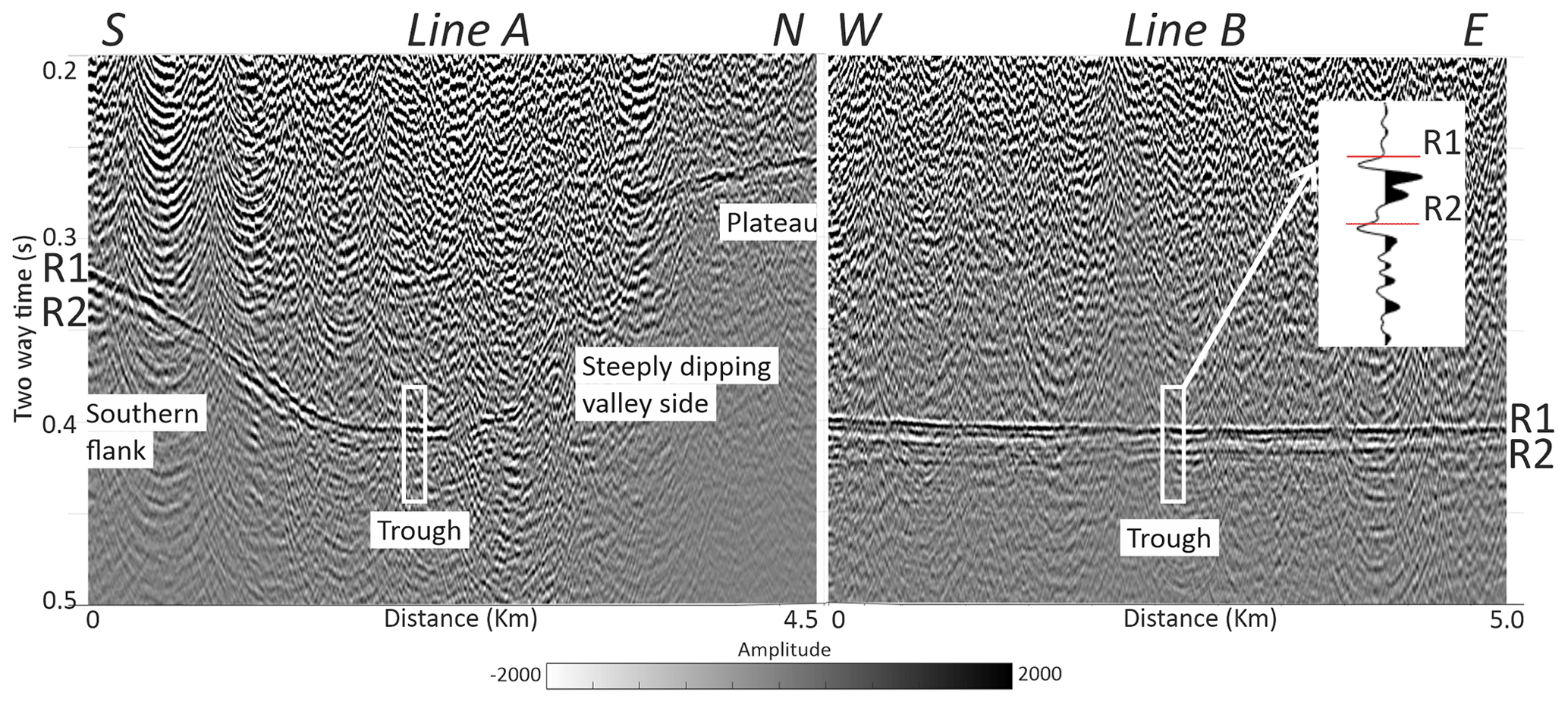
Figure 2 Migrated seismic-reflection sections for line A and B, where the ice–base reflector (R1) is highlighted, and a second reflector, R2, appears directly below in the trough and southern section. The enlarged area shows the seismic signature of R1 and R2.

2.3.1 Arrhenius-modelled attenuation rates

Attenuation rates are derived using the temperature- and chemistry-dependent Arrhenius equation. The derivation and description of Arrhenius-modelled attenuation rates closely follow a previous application over DIC (Rutishauser, 2019). Arrhenius-modelled attenuation rates are derived via the relationship between the radar attenuation rate N_a and the high-frequency limit of the electrical conductivity σ_∞ (measured in µS m⁻¹, Eq. 3), which is related to the ice impurity concentration and temperature via the Arrhenius-type conductivity model (Eq. 4):

$$\begin{array}{}\text{(3)}& N_{\mathrm{a}}={\displaystyle \frac{\mathrm{10}{\log }_{\mathrm{10}}e}{\mathrm{1000}{\mathit{\epsilon }}_{\mathrm{0}}c\sqrt{\mathit{\epsilon }}}}{\mathit{\sigma }}_{\mathrm{\infty }},\end{array}$$

where ε₀ is the permittivity, c is the speed of light in a vacuum, and ε=3.15 is the dielectric permittivity of ice. The Arrhenius conductivity model is expressed as

$$\begin{array}{}\text{(4)}& \begin{array}{rl}{\mathit{\sigma }}_{\mathrm{\infty }}& ={\mathit{\sigma }}_{\mathrm{pure}}\exp \left[{\displaystyle \frac{E_{\mathrm{pure}}}{k}}\left({\displaystyle \frac{\mathrm{1}}{T_{\mathrm{r}}}}-{\displaystyle \frac{\mathrm{1}}{T}}\right)\right]\\ & +{\mathit{\mu }}_{{\mathrm{H}}^{+}}\left[{\mathrm{H}}^{+}\right]\exp \left[{\displaystyle \frac{E_{{\mathrm{H}}^{+}}}{k}}\left({\displaystyle \frac{\mathrm{1}}{T_{\mathrm{r}}}}-{\displaystyle \frac{\mathrm{1}}{T}}\right)\right]\\ & +{\mathit{\mu }}_{{\mathrm{Cl}}^{-}}\left[{\mathrm{Cl}}^{-}\right]\exp \left[{\displaystyle \frac{E_{\mathrm{Cl}}}{k}}\left({\displaystyle \frac{\mathrm{1}}{T_{\mathrm{r}}}}-{\displaystyle \frac{\mathrm{1}}{T}}\right)\right]\\ & +{\mathit{\mu }}_{{\mathrm{NH}}_{\mathrm{4}}^{+}}\left[{\mathrm{NH}}_{\mathrm{4}}^{+}\right]\exp \left[{\displaystyle \frac{E_{{\mathrm{NH}}_{\mathrm{4}}^{+}}}{k}}\left({\displaystyle \frac{\mathrm{1}}{T_{\mathrm{r}}}}-{\displaystyle \frac{\mathrm{1}}{T}}\right)\right],\end{array}\end{array}$$

where σ_pure and E_pure represent the conductivity and activation energy for pure ice, respectively; $k=\mathrm{1.38}\times {\mathrm{10}}^{-\mathrm{23}}$ J K⁻¹ is the Boltzmann constant; T is the ice temperature; and T_r is a reference temperature. For the impurities H⁺, Cl⁻, and NH${}_{\mathrm{4}}^{+}$, μ_x is the molar conductivity, [x] is the molarity, and E_x is the activation energy. Values for the molar conductivities and pure ice conductivity were taken as the M07 σ_∞ model for the Greenland Ice Sheet described in MacGregor et al. (2015) and applied by Jordan et al. (2016). To model attenuation rates over DIC, impurity concentrations were derived as the mean of measured concentrations along a 20 m deep firn core retrieved on DIC in 2015 (Criscitiello et al., 2021). All parameters used in the σ_∞ model are detailed in Table D1 in Appendix D. The temperature–attenuation rate models and application to two example ice temperature profiles are shown in Fig. D1 in Appendix D.

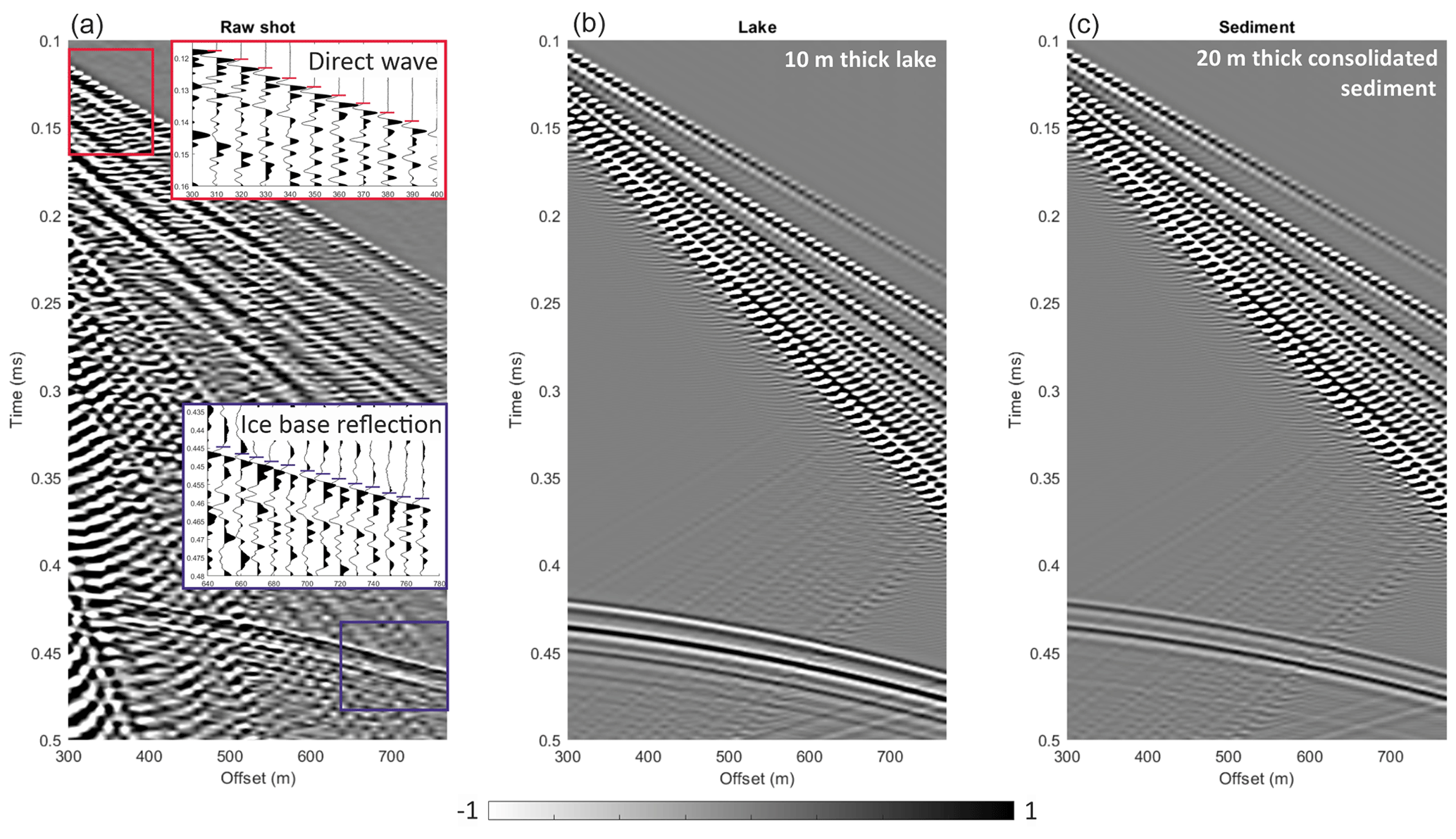
Figure 3 (a) Raw shot gather acquired in the middle of the trough where line A and B cross, thought to be the deepest part of the proposed lake, with enlarged areas of the direct wave and ice–base reflection. (b) Synthetic shot gather of a 10 m thick lake underlying 760 m of glacial ice. (c) Synthetic shot gather of a 20 m thick consolidated sediment package underlying 760 m of glacial ice. The velocity and density models used for these synthetics are shown in Appendix A (Fig. A1).

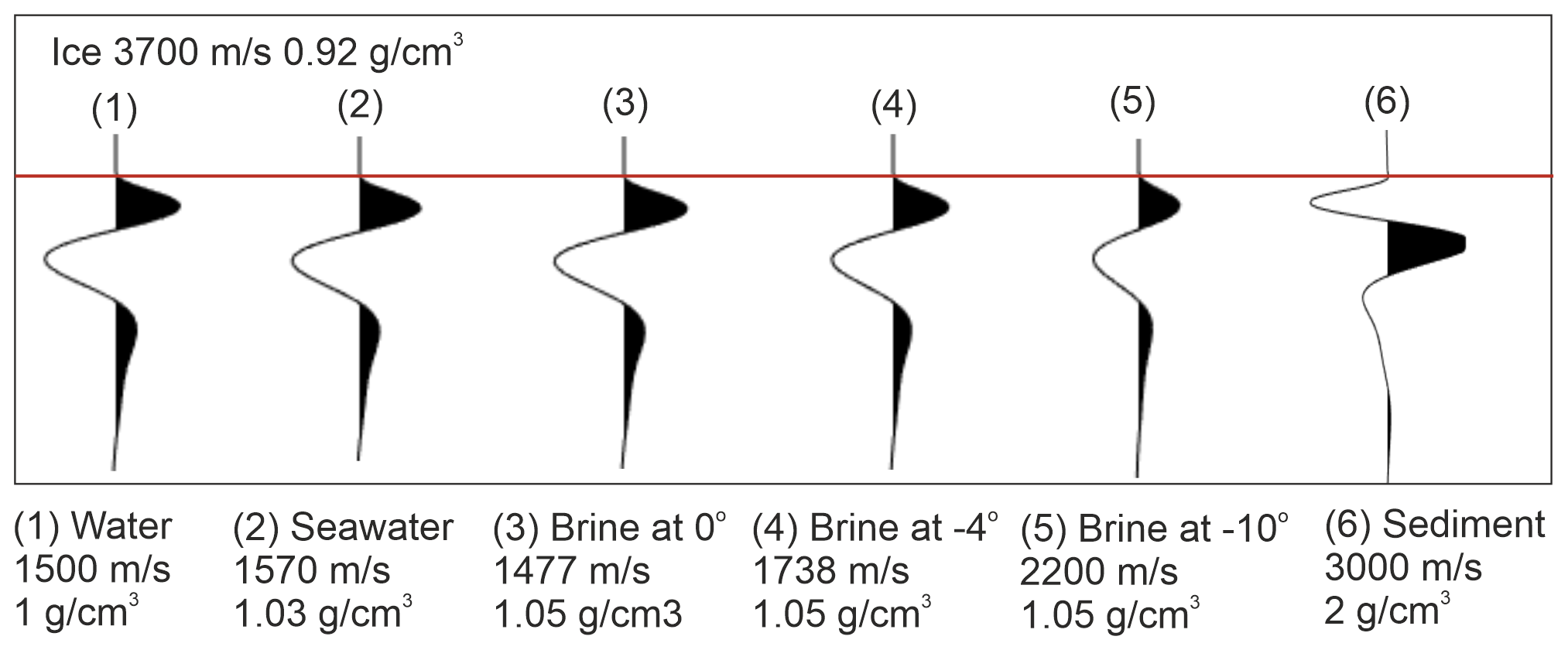
Figure 4 Sensitivity testing for different water types: (1) water (Booth et al., 2012), (2) seawater (Brown, 2016), (3) brine at 0°, (4) brine at −4°, (5) brine at −10°, and (6) consolidated sediment (Peters et al., 2008). The acoustic properties of the brine at different temperatures have come from the results of an acoustic pulse transmission experiment conducted in Prasad and Dvorkin (2004).

Ice temperatures used in the Arrhenius model are estimated from a 1D steady-state advection–diffusion model (Cuffey and Paterson, 2010), previously applied to DIC (Rutishauser et al., 2018, 2022). This temperature model ignores horizontal temperature exchanges as well as basal frictional heating, strain heating from ice deformation, and potential latent heat contributions from refreezing of percolated meltwater in the firn or water at the base of the ice. Flow regime classifications (Burgess et al., 2005) show that the central part of DIC lies within flow regime 1 (FR1, $\frac{v}{d}\le \mathrm{0.05}$ yr⁻¹, where v is the ice surface velocity and d the ice thickness), for which flow is driven by internal deformation, and thus the underlying basic assumptions for a 1D advection–diffusion model are valid.

Ice temperature profiles over DIC are calculated for each grid cell of the ice thickness data by Rutishauser et al. (2022), using a geothermal heat flux of 65 ± 5 mW m⁻² (Grasby et al., 2012), an accumulation rate of 0.19 ± 0.05 m water equivalent per year (Paterson, 1976; Reeh and Paterson, 1988) converted to downward velocity using a firn density of 330 kg m⁻³, and a mean annual air temperature derived via scaling a reference temperature of −23 ± 1 °C at 1825 m a.s.l. (Kinnard et al., 2006) with a 4.1 °C km⁻¹ lapse rate (Rutishauser et al., 2018; Gardner et al., 2009) over the entire ice cap. Finally, data points outside of FR1 ($\frac{v}{d}>\mathrm{0.05}$ yr⁻¹) calculated from velocities reported in Van Wychen et al. (2014) are excluded. Uncertainties from the ice temperature and Arrhenius model are propagated, leading to attenuation rate uncertainties over DIC between 4.6–7.5 dB km⁻¹ and a mean of 6.1 dB km⁻¹ (Fig. D2 in Appendix D).

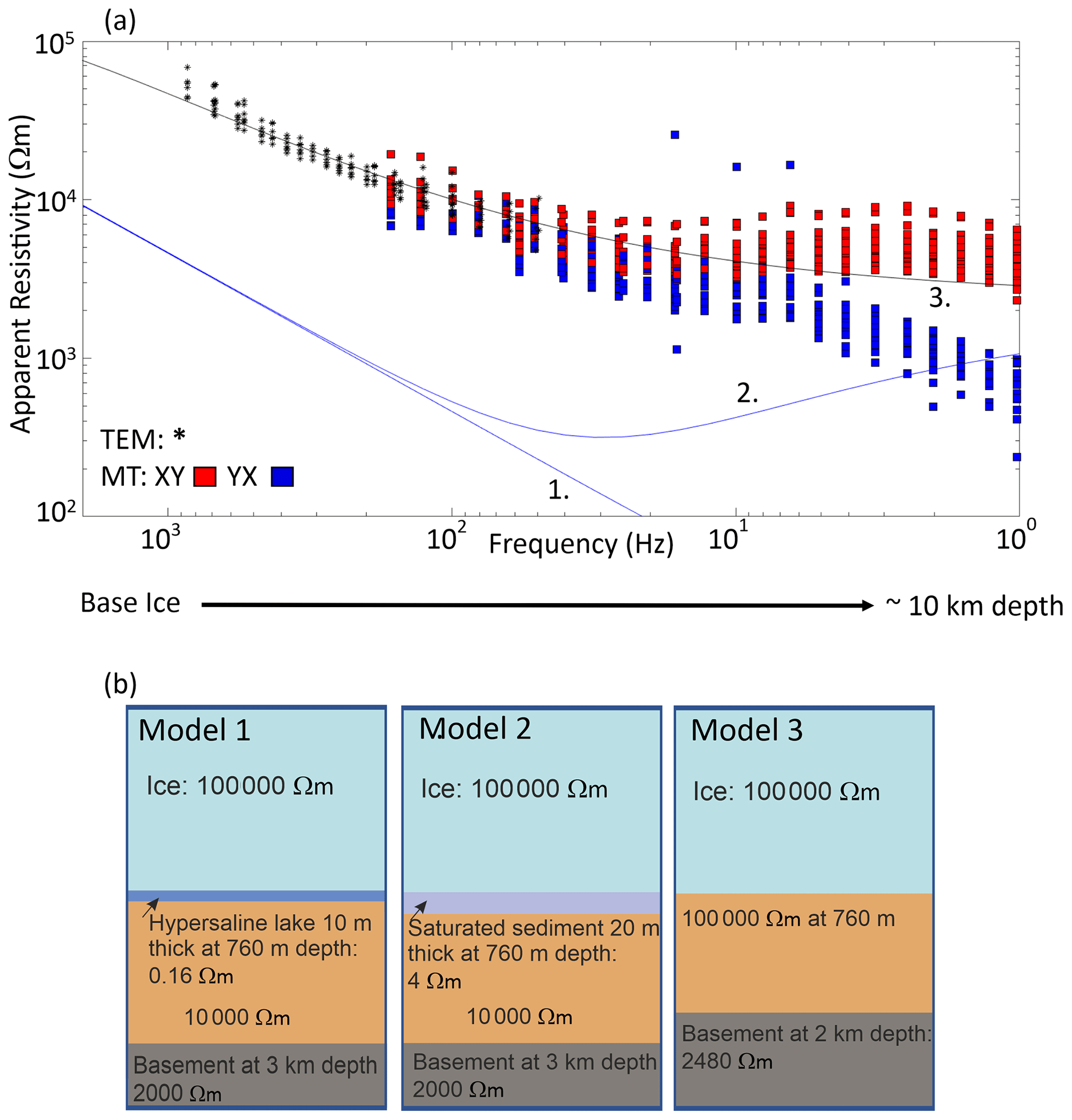
Figure 5 (a) Frequency versus apparent resistivity of the observed TEM and MT data acquired across the whole survey area with synthetic models 1–3 plotted. (b) Resistivity structure of synthetic models 1–3. The time (t) after turn-off for the TEM data has been transformed to the period (T) according to the transformation $T=t/\mathrm{0.2}$, which has been converted to the frequency (f) for the purpose of this plot by $f=\mathrm{1}/T$. For the MT data, the XY data denote apparent resistivity and phase calculated from the north–south electric field and the east–west magnetic field. The YX data denote apparent resistivity and phase calculated from the east–west electric field and the north–south magnetic field.

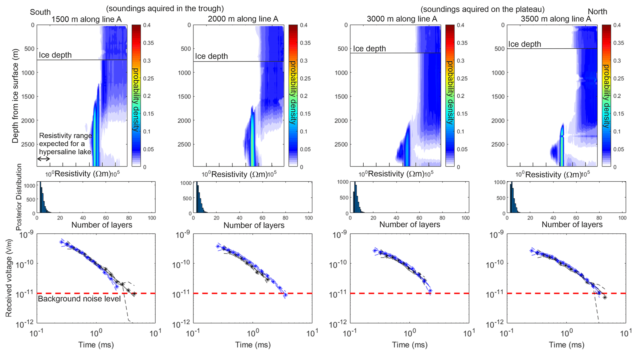
Figure 6 Line A TEM Bayesian inversion results for the 7.5 and 3 Hz base frequencies. Top plot: posterior distribution of resistivity with depth. Middle plot: posterior distribution of the number of layers. Bottom plot: comparison of data fit plot, with the best fitting forward model accepted in the ensemble (–) compared to the data (^*) and error tolerance (– –). The black data points are the 3 Hz base frequency, and the blue data points are the 7.5 Hz base frequency. The dashed red line is the background noise level.

2.3.2 Adaptive attenuation rate fitting

An adaptive bed power to ice thickness fitting approach (Schroeder et al., 2016; Chu et al., 2021) was tested and applied to the radar data (Fig. 12). We use the SRH1 dataset (Rutishauser et al., 2022) and derive attenuation rates at evenly distanced (2.5 km) grid points over the DIC survey area. For each point, we use an initial search radius of 5 km to calculate the correlation coefficient magnitude between the ice thickness and attenuation-corrected bed power for attenuation rates ranging between 0–40 dB km⁻¹. Then, correlation coefficient fit conditions are evaluated, and if not met, the search radius is extended (each round by 1 km) until a maximum radius of 25 km. We set the minimal fit criteria to (1) the minimum correlation coefficient magnitude C_m≤0.01, (2) an initial correlation coefficient magnitude C₀≤0.5, and (3) the radiometric resolution N_h≤3 dB km⁻¹ (Schroeder et al., 2016).

3 Results

3.1 Seismic

The seismic-reflection data clearly image the ice–base reflector (R1) with a second reflector (R2) directly below in the trough and southern section (Fig. 2). In the northern part of line A, a relatively flat plateau is observed with just one primary reflector (R1). Continuing south along line A, the steeply dipping valley side is imaged down to the trough where the lake, T2, was thought to exist. In the trough and southern section, R1 and R2 are observed and clearly separated (maximum separation ∼ 0.013 s). The long-axis profile (line B) clearly images R1 and R2 with constant separation along the trough (∼ 0.011 s).

Here, we define the polarity of the first arrival of the direct wave as positive, identified by a negative minimum-phase wavelet (Fig. 3a). With this in mind, we observe a positive polarity for the ice–base interface (R1) and second reflector (R2) (Fig. 3a). The polarity of R1 is opposite to that expected for subglacial water (Figs. 3b and 4), indicating the material directly under the ice is unlikely to be a lake. Furthermore, if a lake existed in this bedrock trough, the polarity should change at the ice–water and ice–bedrock interfaces along line A, but no polarity reversal is observed between R1 and R2 (Figs. 2 and 3). Using the lake boundaries derived from the RES analysis, we would expect R1 to onlap onto R2 at the lake edge, in the southern part of line A. However, in the southern section of line A, R1 and R2 are clearly separated, with R2 continuing along the southern flank and extending the entire length of line A (Fig. 2).

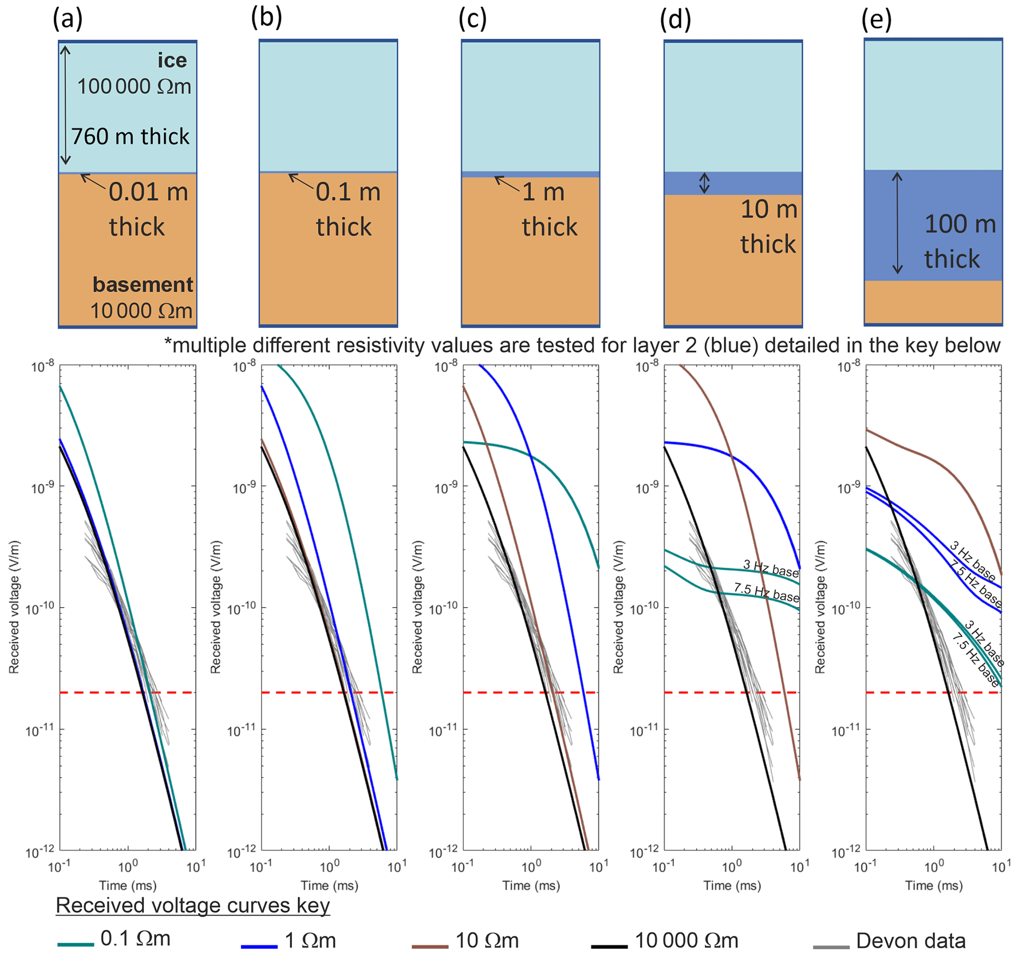
Figure 7 TEM vertical resolution analysis of synthetic three-layered models compared to the DIC TEM data. Synthetic models are shown by the green, blue, brown, and black lines, which include a 100 000 Ω m layer, overlaying a layer with variable thickness and resistivity (0.1, 1, 10, and 10 000 Ω m, respectively) with a 10 000 Ω m basement. The different thicknesses for layer 2 are (a) 0.01 m, (b) 0.1 m, (c) 1 m, (d) 10 m, and (e) 100 m. The DIC TEM data are shown in grey with the background noise levels marked by the dashed red line.

To confirm our polarity analysis, synthetic seismograms were computed using the CREWES finite-difference algorithm (Margrave and Lamoureux, 2019) for two models of (1) a 10 m thick lake underlying 760 m of glacial ice and (2) a 20 m thick consolidated sediment package underlying 760 m of glacial ice (Fig. 3b–c; Appendix A) and compared to the acquired shot gather (Fig. 3a). The source wavelet used in the simulations was a negative minimum-phase wavelet with a dominant frequency of 100 Hz, which best represents our impulse source (hammer and plate) and the direct wave observed in our seismic data. Here, the model of a 20 m thick consolidated sediment package best matches the acquired shot gather (Fig. 3c).

Additionally, we conducted a sensitivity test for the polarity expected at an ice–water interface for different water types: (1) water, (2) seawater, (3) brine at 0°, (4) brine at −4°, and (5) brine at −10° (Fig. 4) (Booth et al., 2012; Brown, 2016; Prasad and Dvorkin, 2004). Our sensitivity testing shows there is always a negative polarity reflection for an ice–water interface for the scenarios tested (Fig. 4). For the ice–brine interfaces, the modelled reflection coefficients ranged from −0.4 for brine at 0° to −0.2 for brine at −10°. Therefore, the positive polarity of R1 is also opposite to that expected for an ice–brine interface.

3.2 Electromagnetics

The observed EM data were compared with synthetic models of (1) a hypersaline lake, (2) saturated sediments, and (3) a resistive subsurface. Here, the observed data have no resemblance to the predictions of the 1D resistivity models representing a hypersaline subglacial lake or saturated sediments. The observed data best fit the model with a very resistive subsurface (> 1000 Ω m) (Fig. 5).

3.2.1 Transient electromagnetics

The results from the 1D MuLTI-TEM inversion for each TEM sounding acquired along line A are shown in Fig. 6. The inverted resistivity profiles of the TEM data show highly resistive rock layers (1000 to 100 000 Ω m) directly under the ice in the trough and on the plateau with a ∼ 1000 Ω m layer at depths > 2 km. Furthermore, all inverted resistivity soundings for line A and B (Appendix B, Fig. B2) show very similar results consisting of a highly resistive subsurface. The TEM method can resolve conductive structures more accurately than resistive ones, highlighted by a tighter probability density function over the lower ∼ 1000 Ω m layer compared to the resistive upper layer shown in Figs. 6 and B2.

Multiple synthetic models were created using the forward-modelling code in MuLTI-TEM. A three-layer model was used with (1) a 100 000 Ω m layer overlaying (2) a layer with variable thickness and resistivity with (3) a 10 000 Ω m basement. The different resistivities tested for layer 2 were 0.1 (representing a hypersaline lake), 1, 10, and 10,000 Ω m. The different thicknesses tested for layer 2 were 0.01, 0.1, 1, 10, and 100 m. Figure 7 shows the results from this test, highlighting that a 0.01 m thick layer of 0.1 Ω m is resolvable compared to the resistive subsurface observed beneath DIC. Also, a 0.1 m thick, 1 Ω m layer, and a 1 m thick, 10 Ω m layer is resolvable compared to the resistive subsurface observed beneath DIC. These results provide further evidence for the lack of subglacial water directly beneath DIC.

3.2.2 Magnetotellurics

At the high frequencies (100–30 Hz), the XY and YX apparent-resistivity curves are similar, suggesting a 1D resistivity structure. Below a frequency of 30 Hz, the XY and YX apparent-resistivity curves separate, indicating a change in resistivity structure to 2D or 3D (Fig. 5a). Here, the phase tensors are aligned with the major axes perpendicular to the trend of the subglacial trough and line B. While the skew angles are not zero, the data in the frequency band 100–1 Hz show evidence for a 2D behaviour with a strike of N105° E (Fig. 8b–c). The data were rotated to a coordinate system with a strike direction of N105° E. The XY data were defined as the TE mode, and the YX data were defined as the TM mode. The measured data show that the TE mode has much lower apparent-resistivity values at low frequency than in the TM mode (Fig. C2).

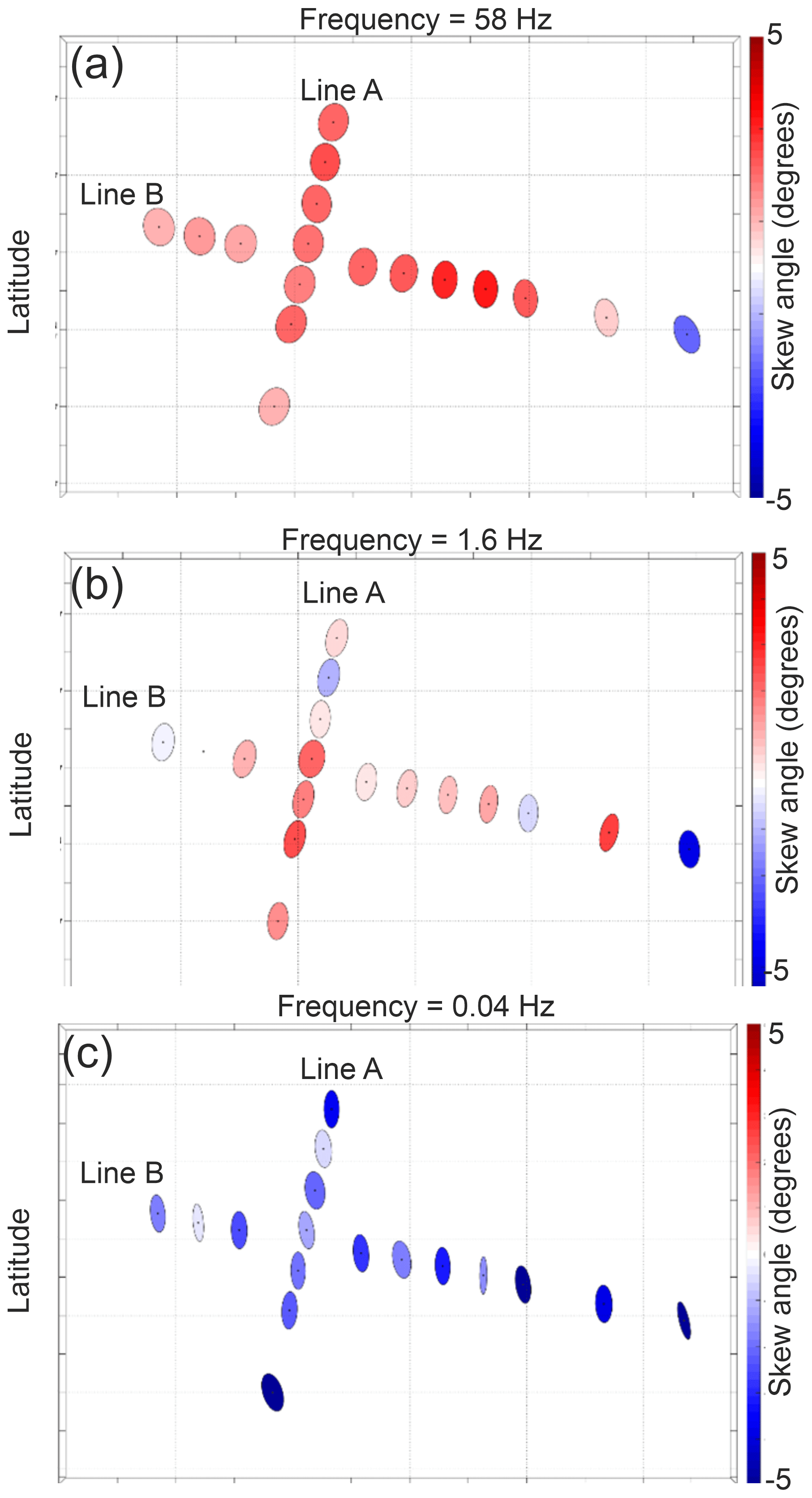
Figure 8 Phase tensor at frequencies of 58, 1.6, and 0.04 Hz plotted in map view. The direction of the major and minor axes of the ellipses show to possible strike directions. Circles indicate a 1D structure, while ellipses indicate a 2D or 3D structure. This direction variation varies with frequency but is consistent with the direction of the trough axis, which is N105° E. The colour fill shows the skew angle of Caldwell et al. (2004). Values close to zero indicate a 1D or 2D resistivity structure. Non-zero values indicate a 3D resistivity structure.

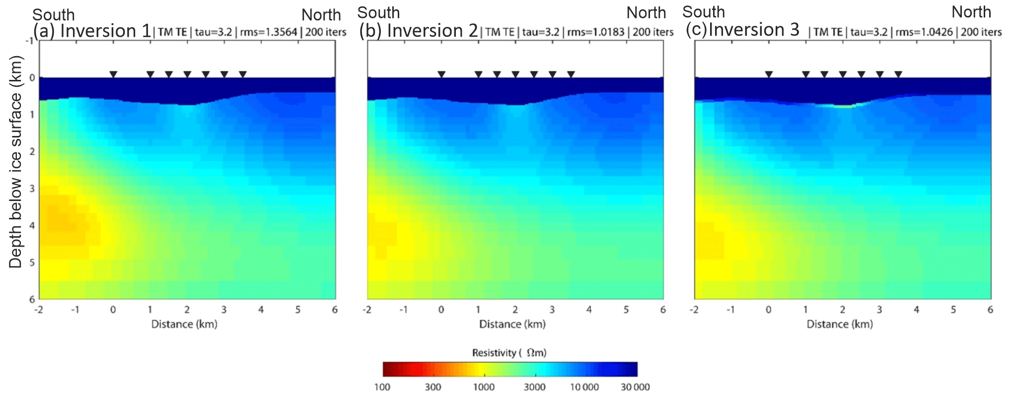
Figure 9 Two-dimensional models for line A obtained by inversion with the algorithm of Rodi and Mackie (2001). The starting model included the ice layer with a resistivity of 100 000 Ω m. (a) Inversion 1. (b) Inversion 2 with static shifts free at the station 1 km along the line. (c) Inversion 3 with statics shifts free at the station 1 km along the line and a second tear added 100 m below the base of the ice. The trade-off parameter for all three inversions was τ=3.2.

Three 2D inversions were undertaken for line A. Line B cannot be inverted with a 2D approach since it is parallel to the geoelectric strike. The first inversion run for line A began from the model with the ice layer. Error floors of 10 % and 5 % were applied to the apparent resistivity and phase, respectively. Data in the frequency band 100–1 Hz were selected for inversion to focus on the shallow structure. The fit is shown in Fig. C2, and good agreement between the measured and predicted MT data can be seen. The final resistivity model is shown in Fig. 9a, where the subglacial resistivity is ∼ 3000–10 000 Ω m, and hypersaline water is expected to have a resistivity of ∼ 0.16 Ω m (Killingbeck et al., 2021). Two features with lower resistivity can be observed in the model. The first is a layer with resistivity in the range 300–1000 Ω m located at a depth of 3–4 km below the surface and dipping to the north. This feature is responsible for the decreasing apparent resistivity as a function of frequency at all stations. The second is a more subtle ∼ 3000 Ω m layer located directly beneath the deepest part of the trough. With the limited number of MT stations, this resistivity feature is only resolved by one or two MT stations. Two additional inversions were performed to determine if this feature is required by the data.

The pseudo-section in Fig. C2 shows evidence for a static shift in the TM apparent resistivity at the station a distance of 1 km along line A. A static shift is a frequency-independent offset in apparent resistivity and is often caused by near-surface heterogeneity. The second inversion for line A allows static shifts to be present in the TE and TM mode data. The second inversion run for line A produced a model that was similar to that obtained in the first inversion (Fig. 9b).

To determine if the relatively low resistivity (∼ 3000 Ω m) basal layer was present beneath the ice, a final inversion was performed with a second tear permitted at a depth of 100 m beneath the base of the ice. This third inversion showed that a ∼ 3000 Ω m layer was consistent with the data but not required (Fig. 9c). The lack of high-frequency MT data limits the resolution of the shallowest subglacial structure that can be resolved. However, these higher frequencies were obtained from the TEM data, and a joint comparison of the measured TEM and MT data with synthetic models showed the observed EM data are very different to that expected for a subglacial hypersaline lake (Fig. 5).

3.3 Properties of the material directly under DIC

The acoustic impedance of the material in the trough, directly beneath the centre of DIC, is estimated using the normal incident reflection coefficient method. Here, the estimated acoustic impedance of reflector R1 is 9.49 ± 1.92 × 10⁶ kg m⁻² s⁻¹, comparable to the hardest rocks and frozen sediments at subglacial Lake Ellsworth, Antarctica (Smith et al., 2018), and significantly higher than that of water at 1.5 × 10⁶ kg m⁻² s⁻¹ (Fig. 10a). Laboratory studies which measured the acoustic properties of permafrost samples collected in the Canadian Arctic show that an increase in clay content results in a decrease in seismic velocity at temperatures < 0 °C (King, 1984). An increase in porosity and pore fluid salinity can lead to a decrease in the seismic velocity at temperatures < 0 °C (Pandit and King, 1979). Direct comparison of these studies to the estimated acoustic impedance of the subglacial material in the trough beneath DIC suggests the material could have a low clay content and a low content of unfrozen saline pore fluid (Fig. 10a).

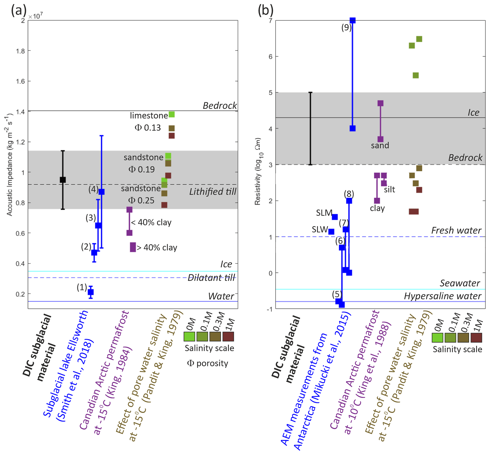
Figure 10 Properties of the material in the trough directly beneath DIC. (a) Acoustic impedance compared to that of subglacial material from subglacial Lake Ellsworth – (1) lake bed, subaqueous, and soft wet sediment; (2) subglacial and soft wet sediments; (3) hard bed and wet sediments; and (4) hardest bed, rock, or frozen sediment (Smith et al., 2018) – as well as laboratory studies measuring the acoustic properties of permafrost and sedimentary samples collected in the Canadian Arctic at −15 °C (King, 1984; Pandit and King, 1979). Horizontal coloured lines represent estimated acoustic impedance values for different materials detailed in Peters et al. (2008). (b) Resistivity compared to that of subglacial Lake Whillans (SWL; Christner et al., 2014) and subglacial Mercer Lake (SLM; Priscu et al., 2021) direct samples – airborne electromagnetic (AEM) measurements from the Taylor dry valley, Antarctica; (5) Blood Falls outflow; (6) west Lake Bonney between 5 m and 35 m depth; (7) Lake Fryxell between 5 m and 18 m depth; (8) sediments with brine in the pore; and (9) glacier ice (Mikucki et al., 2015) – as well as laboratory studies measuring the resistivity of permafrost and sedimentary samples collected in the Canadian Arctic at a temperature of $<-\mathrm{10}$ °C (Pandit and King, 1979; King et al., 1988). Horizontal coloured lines represent estimated resistivity values for different materials detailed in Killingbeck et al. (2021) and Key and Siegfried (2017).

The inverted resistivity profiles of both the TEM and MT measurements suggest highly resistive rock layers (1000–100 000 Ω m) are present directly beneath the ice, with a 1000 Ω m layer at depths > 2 km (Figs. 6, 9 and B2). These resistivity values are ∼ 3 orders of magnitude greater than those expected in the presence of a hypersaline lake (∼ 0.16 Ω m; Killingbeck et al., 2022), a freshwater lake (1–10 Ω m; Christner et al., 2014; Priscu et al., 2021), or unfrozen saturated sediment (∼ 1–100 Ω m; Gustafson et al., 2022) (Fig. 10b). At temperatures $<-$10 °C, a high clay content and saline pore fluid can decrease the resistivity by orders of magnitude (Pandit and King, 1979; King et al., 1988). Direct comparison of these studies to the estimated resistivity of the subglacial material in the trough beneath DIC supports our interpretation from the acoustic impedance analysis that the material is likely to have a low clay content and low content of unfrozen saline pore fluid.

3.4 Re-evaluation of the RES reflectivity data

The Arrhenius-modelled attenuation rates over DIC range between 14–23 dB km⁻¹, with a mean of 17 dB km⁻¹ along all survey lines and 15.6 dB km⁻¹ over the lake area (Fig. 11). These attenuation rates are significantly lower than the radar-derived attenuation rates (Fig. 11a), and applying them to correct the returned bed power yields a much lower basal reflectivity in the trough (5.7 and 3.2 dB, respectively, Fig. 11d, Table 1). These lower reflectivities do not meet the basal reflectivity threshold expected for the presence of subglacial water (Carter et al., 2007) and would have not led to the interpretation of a subglacial lake.

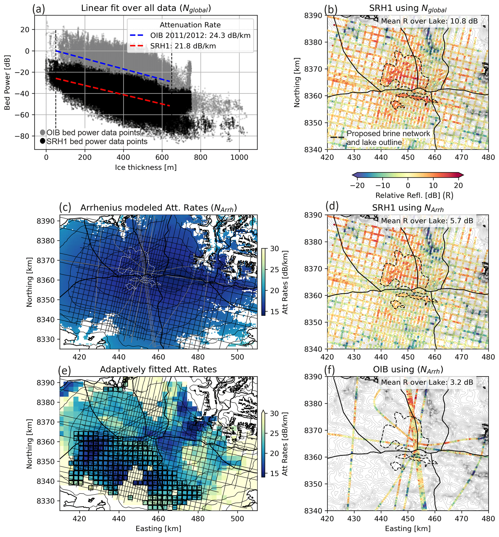
Figure 11 Reanalysis of radar attenuation rates and reflectivity over DIC. (a) Linear regression fits (over the entire DIC datasets) to derive attenuation rates (N_global) from the Operation IceBridge (OIB) MCoRDS radar data (2011, 2012) used in Rutishauser et al. (2018) (grey) and the SRH1 HiCARS data used in Rutishauser et al. (2022) (black). (b) SRH1 basal reflectivity (Rutishauser et al., 2022) corrected using a constant (N_global) rate of 21.8 dB km⁻¹ (linear regression in panel a). (c) Arrhenius-modelled attenuation rates over DIC. Thin black and grey lines are the SRH1 and OIB 2011/2012 survey lines, respectively. (d) SRH1 basal reflectivity corrected using the Arrhenius-modelled attenuation rates (N_Arrh, shown in panel c). (e) Attenuation rates derived from the SRH1 dataset via an adaptive fitting approach (Schroeder et al., 2016b; Chu et al., 2021). Black squares indicate areas where the minimum fit criteria are not met (Appendix D). (f) OIB 2011/2012 basal reflectivity corrected using the Arrhenius-modelled attenuation rates (shown in panel c). All attenuation rates are noted as one-way attenuation rates.

Table 1 Comparison of radar-derived and Arrhenius-modelled attenuation rates (one-way) over DIC, including the resulting mean basal reflectivity (R) over the previously hypothesized subglacial lake area.

Applying the adaptive bed power to ice thickness method, the attenuation rates are shown to increase towards the margins (Fig. D3 in Appendix D), which is a reasonable result. However, the spatial distribution reveals abrupt transition zones that may be artefacts of the method rather than abrupt changes in the ice properties. Furthermore, the minimum fitting criteria are not met over most of the southern catchment area on DIC, including the hypothesized subglacial lake region, highlighting the difficulties in applying this method to the DIC RES dataset.

4 Conclusions

In this study, we provide new geophysical evidence which shows that the proposed hypersaline subglacial lake beneath DIC is unlikely to contain water and has been misidentified. Seismic analysis shows that the ice–base interface in the location of the proposed lake has a positive reflection, and the acoustic impedance of the material is estimated to be 9.49 ± 1.92 × 10⁶ kg m⁻² s⁻¹, comparable to the hardest rocks and frozen sediments at subglacial Lake Ellsworth, Antarctica. The inverted resistivity profiles of both the TEM and MT measurements suggest highly resistive rock layers (1000–100 000 Ω m) directly under the ice, comparable to Arctic permafrost and bedrock. Re-evaluation of the airborne reflectivity data at DIC shows that the RES attenuation rates (derived directly from the RES data via a linear regression fit between the observed bed power and ice thickness) were likely overestimated, leading to an overestimation of the basal reflectivity in the original RES studies (10.8 dB mean over the lake). Here, we derived new attenuation rates using the temperature- and chemistry-dependent Arrhenius equation and applied them to correct the returned bed power. Our new analysis shows the bed power (5.7 dB mean over the lake) does not meet the basal reflectivity threshold expected over subglacial water. At present, a set of criteria need to be met for a subglacial lake to be identified using RES datasets. Most often, the identification of a subglacial lake is made based on relatively high basal RES reflectivity and specularity content and lying in a hydraulically flat region (Carter et al., 2007). This important example shows that the detection of subglacial lakes by RES is highly sensitive to the attenuation rate applied. We show different methods for calculating attenuation rates may yield different basal reflectivities and should be rigorously assessed during RES analysis. Evidently, sensitivity studies on radar attenuation rates are a critical step in RES processing and are fundamental to accurately identify subglacial lakes. We suggest the current criteria for subglacial lake detection from RES datasets include an attenuation rate sensitivity assessment to quantify uncertainty in the basal reflectivity. Furthermore, we suggest a move towards reporting RES-proposed subglacial lakes probabilistically or using confidence levels, e.g. Bowling et al. (2019). Finally, our study highlights that the acquisition of multiple geophysical techniques, where logistically possible, is essential to reliably interpret subglacial water systems.

Appendix A: Active-source seismic-reflection synthetic modelling

For our synthetic seismograms, the near-surface Vp structure of the snow, firn, and ice was derived from refraction observations in the seismic data, where the travel times of the first arrivals were picked and a tomography inversion was applied. This was used as the shallow Vp profile (0–80 m) of the synthetic models. The seismic velocity profiles for the two models are shown in Fig. A1a and b.

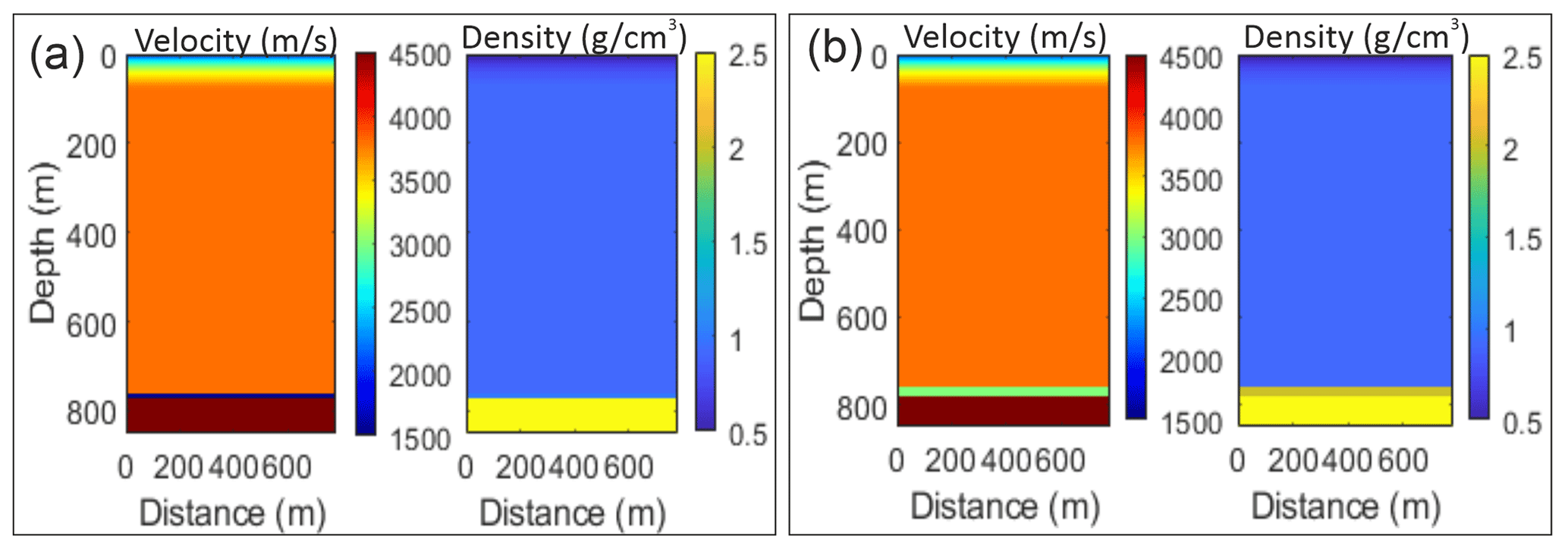
Figure A1 (a) Vp and density model used to compute the synthetic model shown in C. (b) Vp and density model used to compute the synthetic model shown in D.

Appendix B: Transient electromagnetics

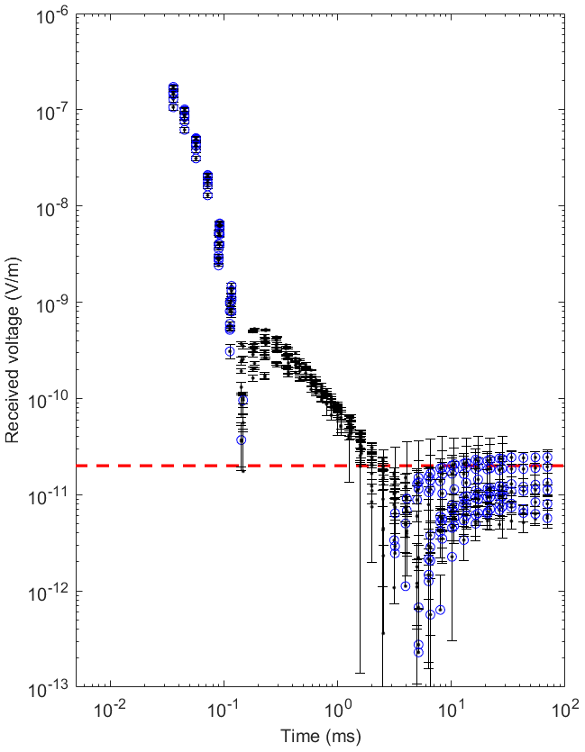
Figure B1 Raw TEM data for all soundings with error bars. Blue circles are negative received voltages, and black dots are positive received voltages. The red line indicates the estimated background noise level.

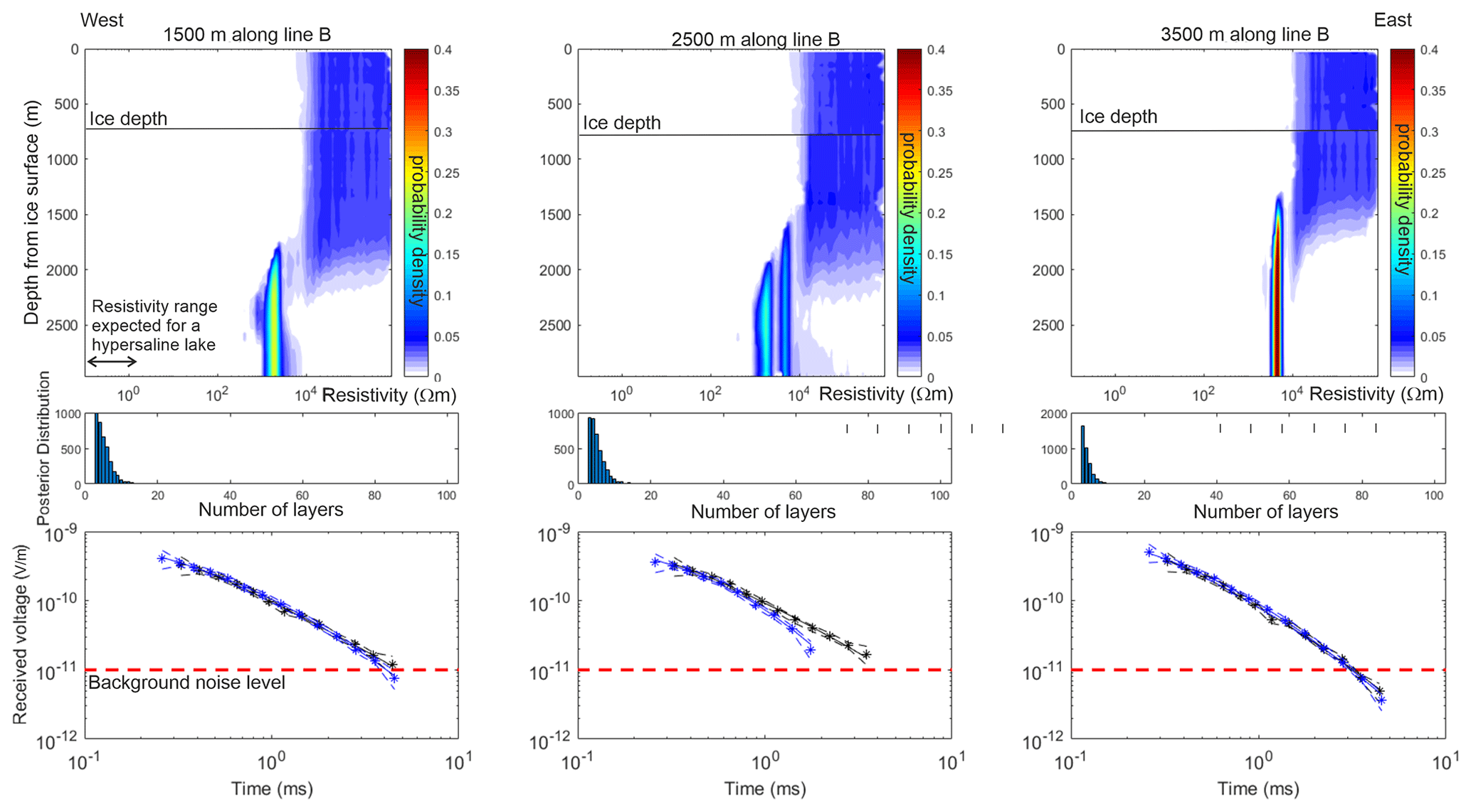
Figure B2 Line B TEM Bayesian inversion results for the 7.5 and 3 Hz base frequencies. Top plot: posterior distribution of resistivity with depth. Middle plot: posterior distribution of the number of layers. Bottom plot: comparison of data fit plot, with the best fitting forward model accepted in the ensemble (–) compared to the data (^*) and error tolerance (– –). The black data points are the 3 Hz base frequency, and the blue data points are the 7.5 Hz base frequency. The dashed red line is the background noise level.

Table B1 TEM survey parameters input into MuLTI-TEM (Killingbeck et al., 2020).

Table B2 MuLTI-TEM inversion parameters.

Appendix C: Magnetotellurics

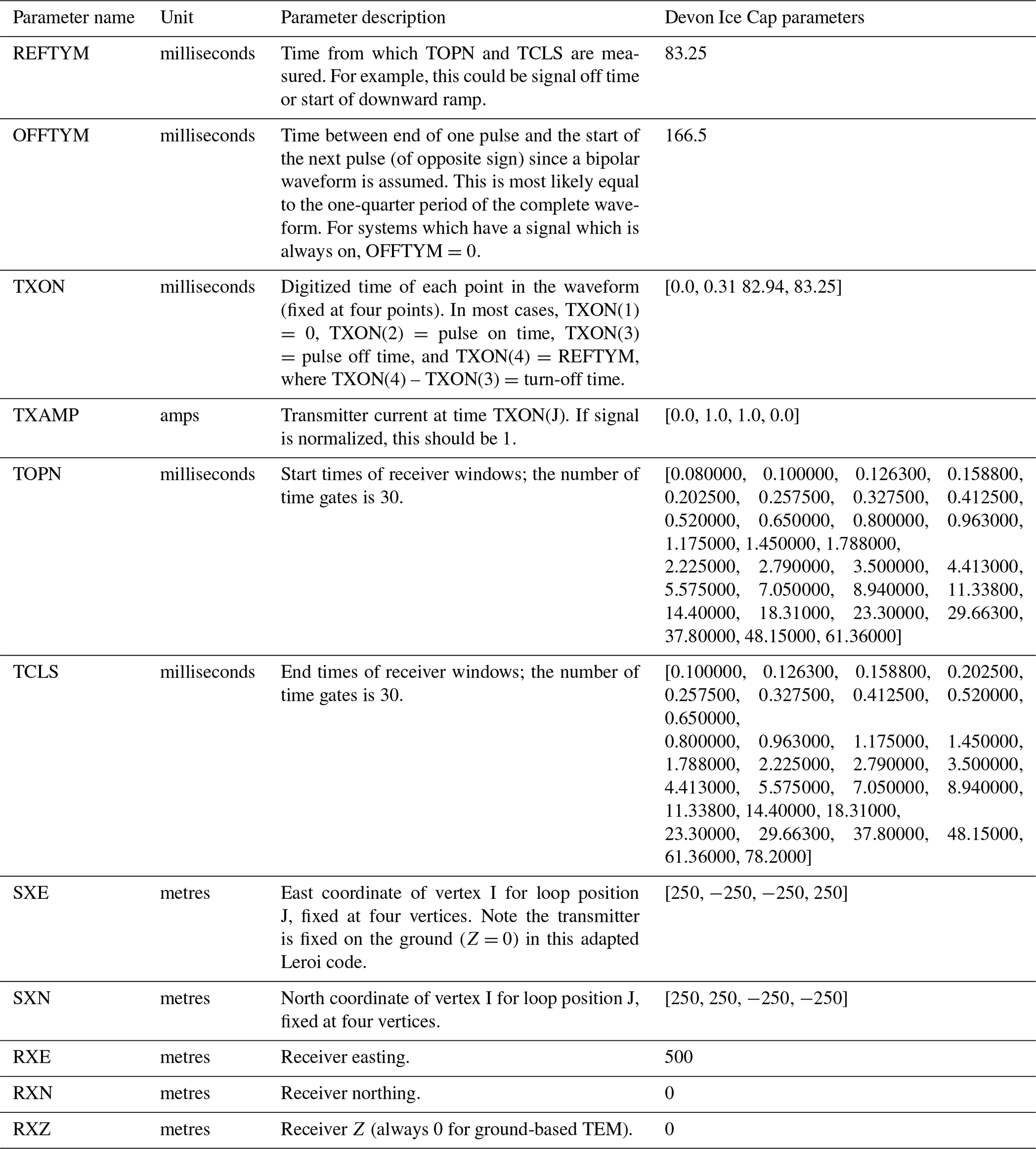
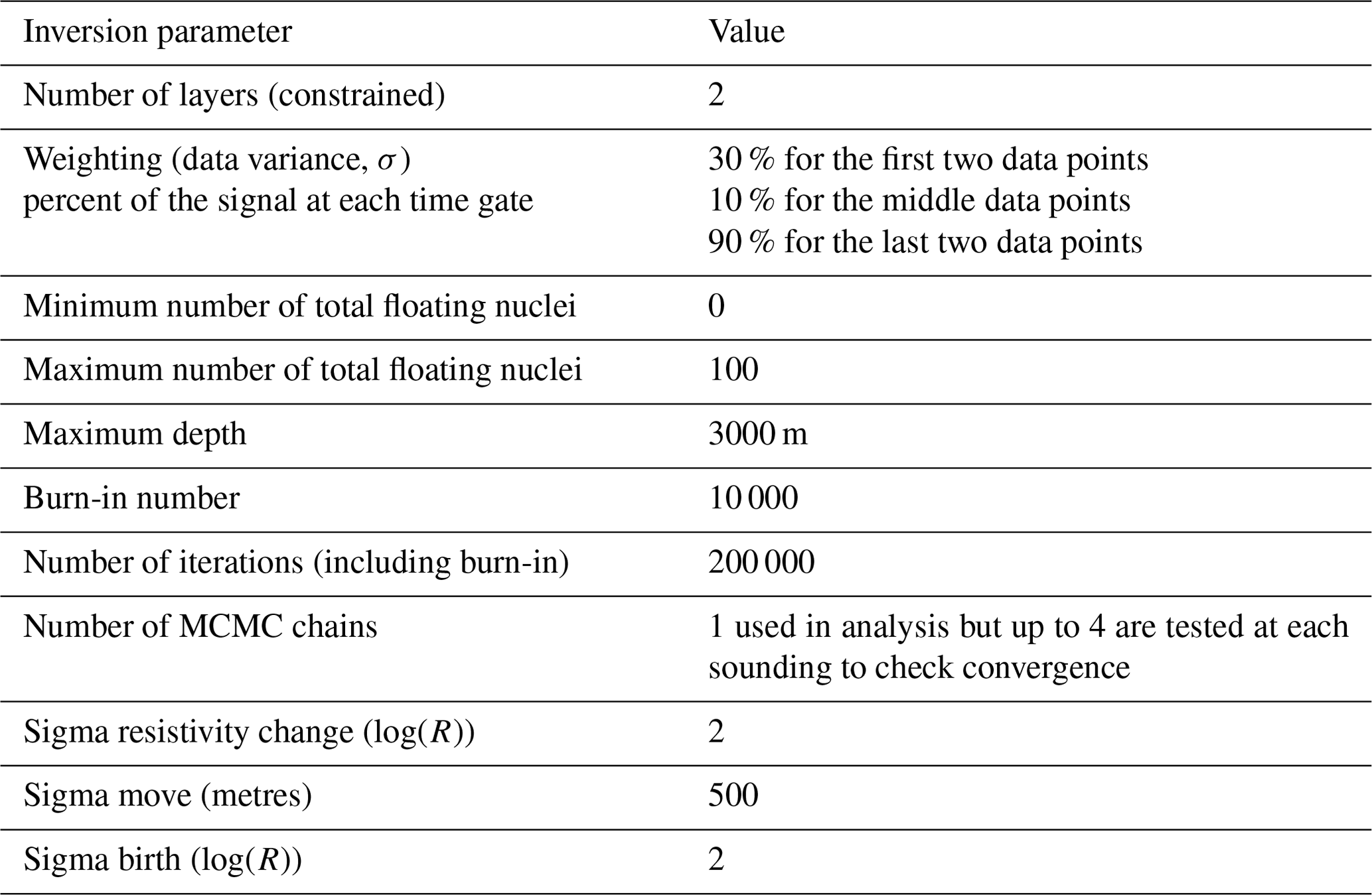
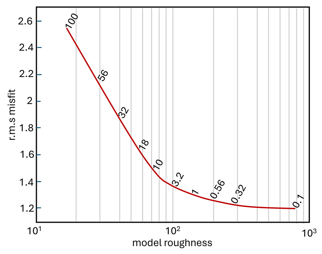
Figure C1 L curve for inversion 1. A value of τ=3.2 represents a compromise between reducing the rms misfit (error-weighted value) as much as possible and preventing the resistivity model from over fitting the data. The τ=3.2 inversion reached an rms misfit of 1.356 after 200 iterations. The rms misfit is the error weighted value, where an ideal fit would result in a value of 1.

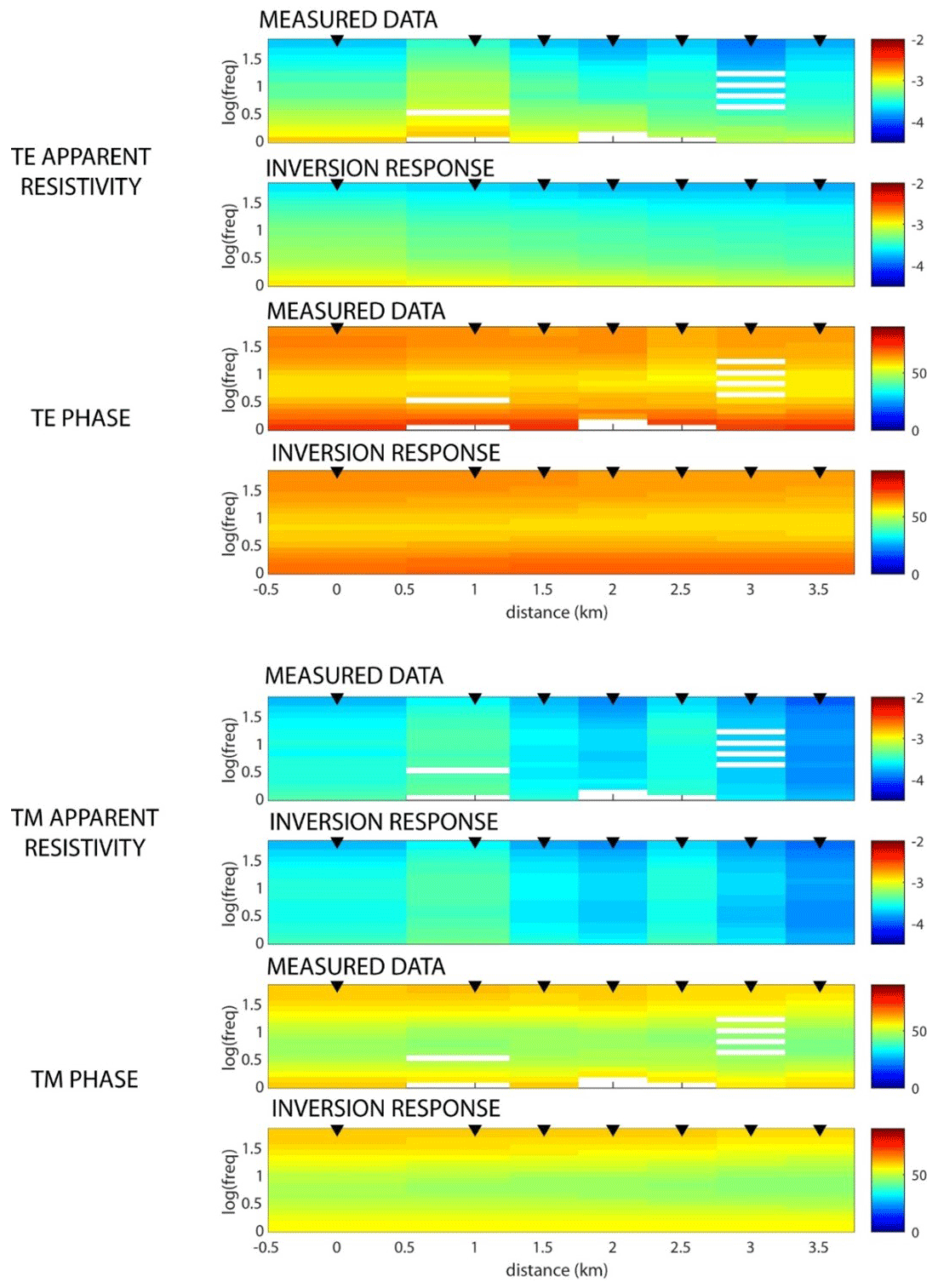
Figure C2 Pseudo-sections of the MT data of line A rotated to a coordinate system with × = N105° E. Each data quantity is compared to the predicted inversion response of inversion 1 with τ=3.2 after 200 iterations.

Appendix D: Re-evaluation of the airborne reflectivity

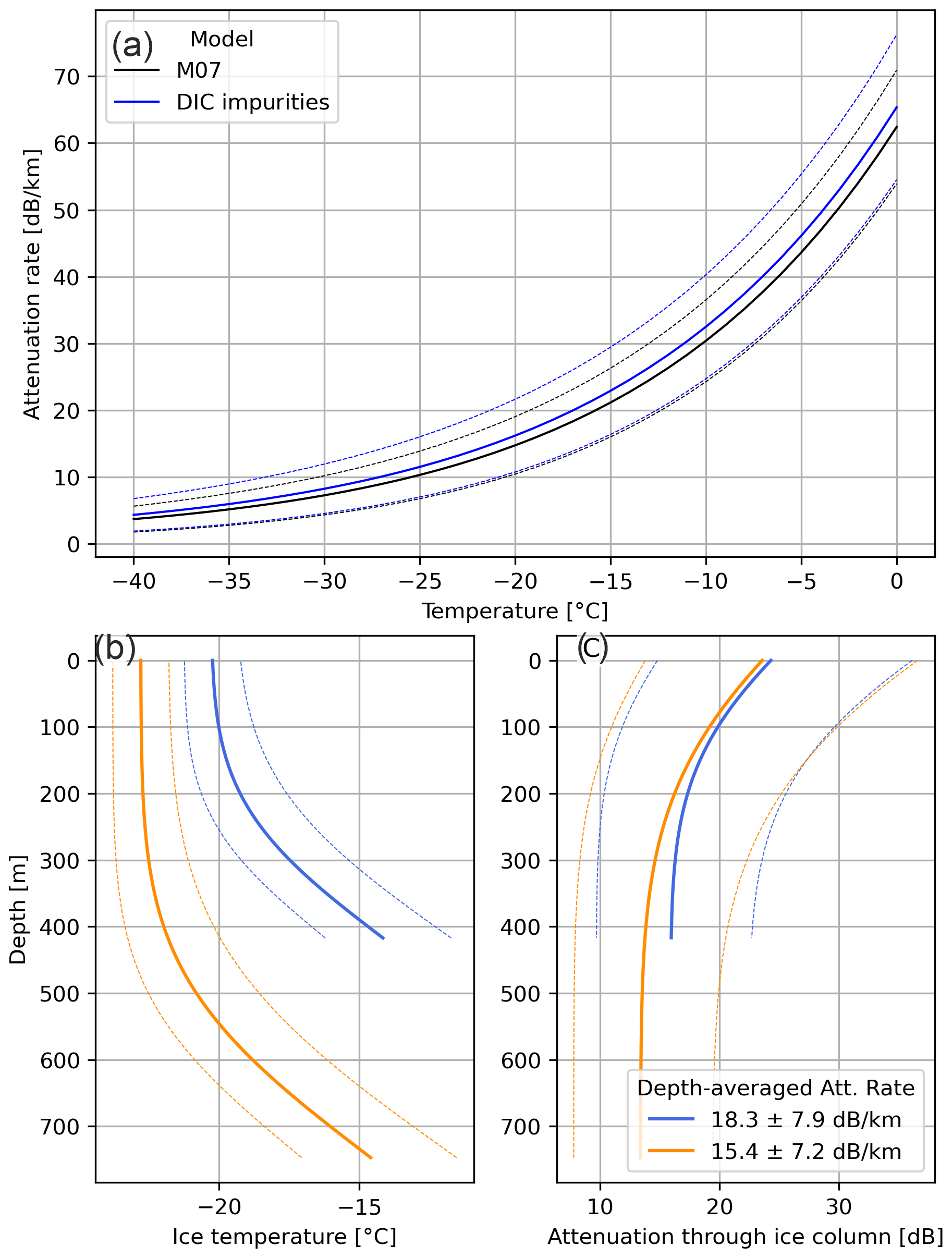
Figure D1 (a) Attenuation rate as a function of ice temperature from the models used over DIC and Greenland (M07). (b) Example ice temperature profiles including their uncertainty ranges, and (c) resulting attenuation rates (one-way) through the ice column, propagating ice temperature and impurity uncertainties.

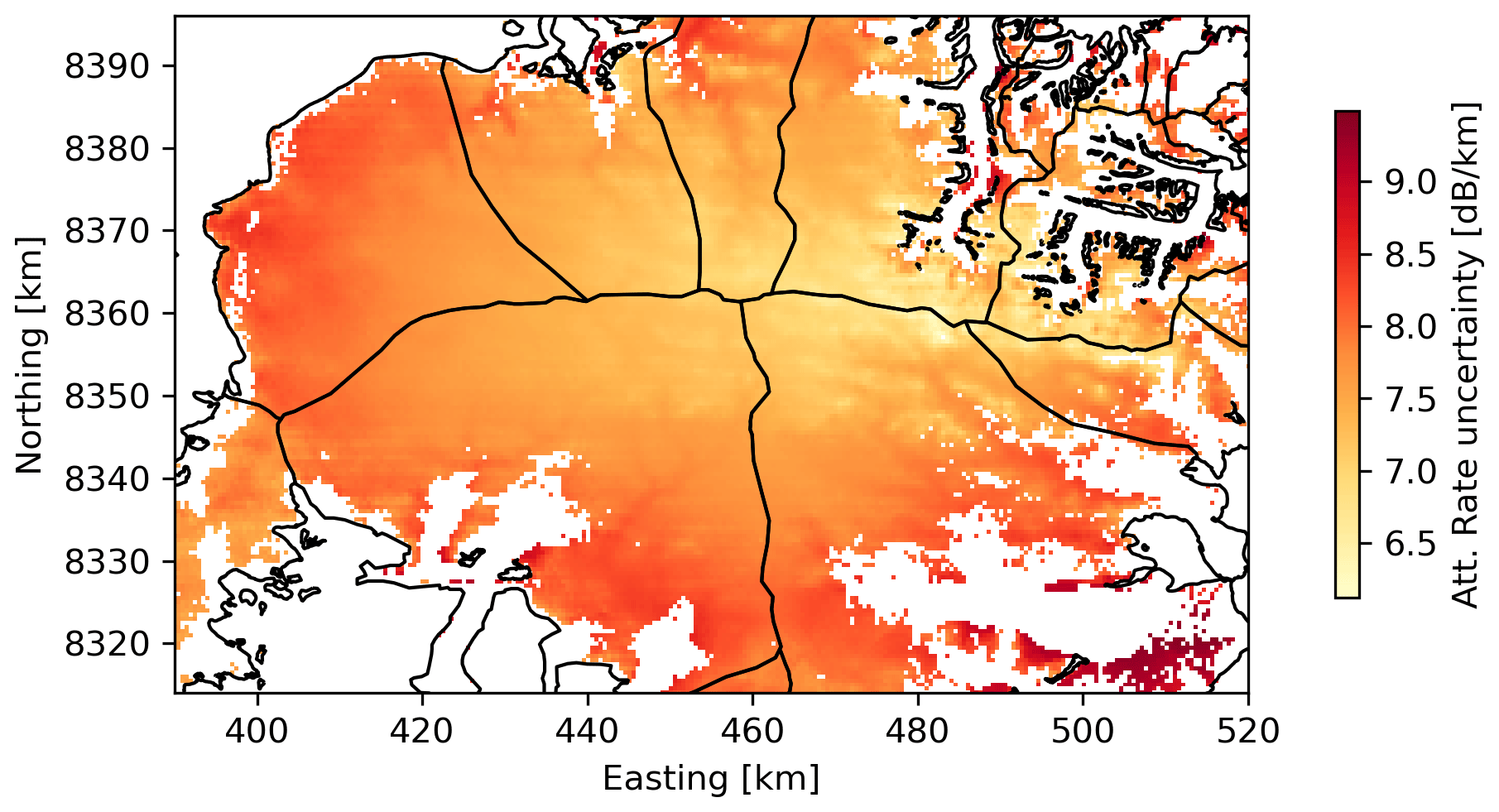
Figure D2 Uncertainty of Arrhenius-modelled attenuation rates over DIC.

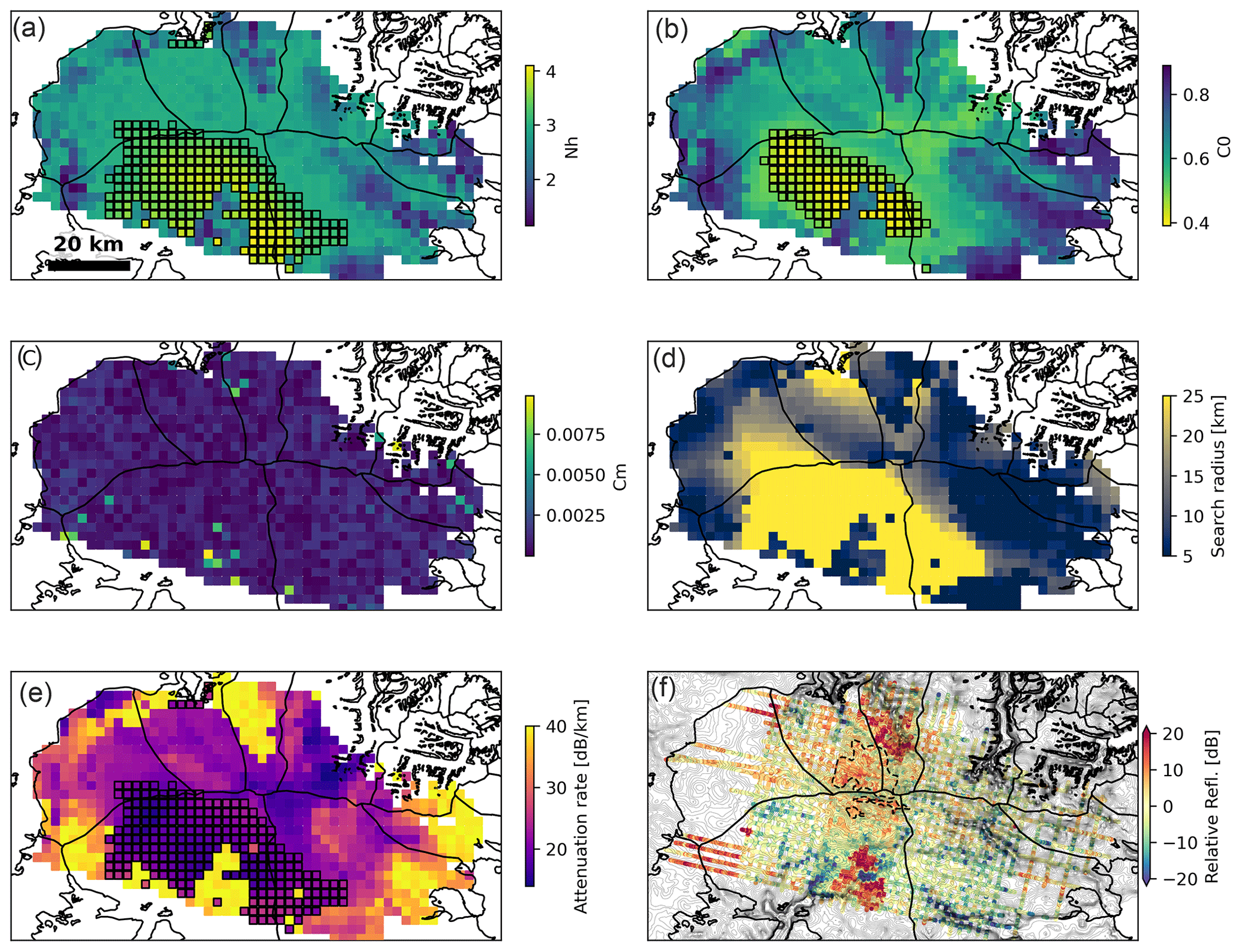
Figure D3 Results and correlation fit parameters from the adaptive attenuation fitting approach (Schroeder et al., 2016b; Chu et al., 2021). (a) Half width of the correlation coefficient minimum N_h. (b) Uncorrected correlation coefficient magnitude C₀. (c) Minimum correlation coefficient C_m. (d) Search radius used to derive the resulting attenuation rate (either the criteria are met or the maximum search radius of 25 km is reached). (e) One-way attenuation rate. Black squares mark areas where the minimum fit criteria of N_h ≤ 3 dB km⁻¹ (a) or C₀ ≥ 0.5 (b) are not met. (f) Relative basal reflectivity upon application of the attenuation rates in panel (e).

Table D1 Parameters used in the Arrhenius-type conductivity model to estimate attenuation rates across DIC and over the NW Greenland subglacial lakes.

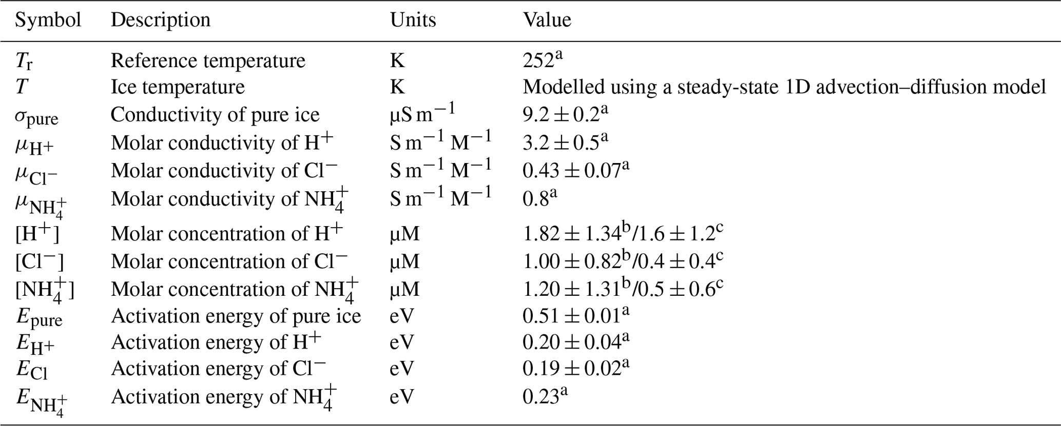
^a Values taken from the M07 model for the Greenland Ice Sheet as described in MacGregor et al. (2015) and applied by Jordan et al. (2016). ^b Average concentration measured along a DIC firn core (Criscitiello et al., 2021) and used for the Arrhenius attenuation rate model over DIC. H⁺ is derived from the HNO₃ concentrations. ^c Impurity concentrations during the Holocene epoch used by MacGregor et al. (2015).