Dynamic and thermodynamic processes related to sea-ice surface melt advance in the Laptev Sea and East Siberian Sea

Arctic summer sea ice has shrunk considerably in recent decades. This study investigates springtime sea-ice surface melt onset in the Laptev Sea and East Siberian Sea, which are key seas along the Northeast Passage. Instead of region-mean melt onset, we define an index of melt advance, which is the areal percentage of a sea that has experienced sea-ice surface melting before the end of May. Four representative scenarios of melt advance in the region are identified. Each scenario is accompanied by a combination of distinct patterns between atmospheric circulation, atmospheric thermodynamic state, sea-ice cover (polynya activity), and surface energy balance in May. In general, concurrent with faster melt advance are a warmer and wetter atmosphere, less sea-ice cover, and surface energy gains in spring. Melt advance can be potentially used in the practical seasonal prediction of summer sea-ice cover. This study suggests the interannual and interdecadal flexibility of spring circulation in the lower troposphere and the significance of seasonal evolution in the Arctic.

1 Introduction

Since the 1970s, satellites have enabled global detection of the Earth. Arctic summer sea-ice extent is found to have decreased dramatically in the past 4 decades (Petty et al., 2020; Stroeve and Notz, 2018), which is a prominent indicator of global warming. In fact, the Arctic has a faster warming trend than elsewhere on the planet, especially in the lower troposphere during the cold season (Cohen et al., 2014; Serreze et al., 2009; Screen and Simmonds, 2010). This phenomenon, called Arctic Amplification, presumably results from reduced sea-ice cover and enhanced oceanic energy release toward the atmosphere, atmospheric and oceanic heat transport from lower latitudes, and local positive feedback (Serreze et al., 2009; Cohen et al., 2014; Taylor et al., 2022). Some research has indicated that the midlatitudes may frequently experience severe winters due to the Arctic Amplification, which reduces the meridional temperature gradient and in turn amplifies the planetary Rossby wave and makes it more stationary (Francis and Vavrus, 2015). In the Arctic, positive ice–albedo feedback is active in the melt season (Budyko, 1969; Kashiwase et al., 2017; Sellers, 1969); after sea ice begins to melt in spring, surface albedo decreases substantially, which favors more solar radiation absorption and promotes further sea-ice melting. Based on this idea, some studies have tried to predict Arctic summer sea-ice cover by sea-ice surface melt onset (MO) in spring, i.e., the date when the sea-ice surface begins to form liquid water (Petty et al., 2017; Wang et al., 2011). Currently, satellite remote sensing helps us construct the pan-Arctic sea-ice MO, which is not possible with only in situ field observations. However, for sea-ice lateral and bottom melting, satellites are less useful and buoys are widely employed (Lei et al., 2022).

Many studies have touched on sea-ice MO in springtime (Drobot and Anderson, 2001; Bliss and Anderson, 2014; Horvath et al., 2021; Crawford et al., 2018; Markus et al., 2009; Stroeve et al., 2014). Generally, sea-ice MO is becoming earlier in most parts of the Arctic, which is consistent with Arctic warming. Another notable feature of MO is its regionality. For example, the Barents Sea, Kara Sea, Laptev Sea, and East Siberian Sea are around the same latitudes along the Siberian coast, but the MO trends were −7.1, −5.2, −2.8, and −1.8 d per decade from 1979 to 2013, respectively (Stroeve et al., 2014). Liang and Su (2021) investigated the interannual early–late relationship of MO between the Laptev Sea and East Siberian Sea, which is related to the large-scale atmospheric pattern of the Barents Oscillation (Skeie, 2000). Locally, synoptic processes are regarded as responsible for interannual variability. Mortin et al. (2016) argued that sea-ice MO is generally associated with higher surface air temperature (SAT), total column water vapor (TWV), and cloud cover, which promotes downward longwave radiation.

The Laptev Sea (LS) and East Siberian Sea (ESS) are marginal seas of the Arctic Ocean, north of Siberia along the Northeast Passage (Fig. S1 in the Supplement). The longitude–latitude ranges are around 70–80° N and 100° E–180°, covering 0.66 and 1.14×10⁶ km² for the LS and ESS, respectively. These two seas are among the regions where sea-ice decline in September during the past 4 decades has been the most prominent, and they are key regions for safe transportation across the Northeast Passage. In spring, sea ice almost completely covers the seas, while in summer, sea ice retreats substantially away from the coast.

Focusing on the LS and ESS, which usually have the most persistent sea-ice coverage in the Northeast Passage, this study aims to demonstrate the springtime processes related to different melt advance scenarios and explore the linkage between springtime melt advance and summertime sea-ice coverage.

2 Data and methods

Sea-ice melt onset (MO) is the date when the sea-ice surface begins to melt in spring, which is retrieved from satellite passive microwave signals (Markus et al., 2009). Liquid water has greater emissivity than ice and snow, so surface melting invokes changes in passive microwave signals. The dataset is distributed by the National Aeronautics and Space Administration (NASA) Cryospheric Sciences Research Portal. We use the yearly MO from 1979 to 2018 with a spatial resolution of ∼ 25 km. Following the method in Liang and Su (2021), we fill in the missing MO values based on surface air temperature (SAT) datasets from the International Arctic Buoy Programme/Polar Exchange at the Sea Surface (IABP/POLES) for 1979–2004 and the Atmospheric Infrared Sounder (AIRS) for 2005–2018. Although there are few missing values, the analysis here is more convenient if the whole research area in the LS and ESS is covered.

The sea-ice concentration (SIC) dataset, called the Ocean and Sea Ice Satellite Application Facility (OSI SAF), is from the European Organization for the Exploitation of Meteorological Satellites (EUMETSAT; Lavergne et al., 2019). We use the monthly SIC in May from 1979 to 2018, with a resolution of 25 km. We also examine SIC dataset from the NASA Team algorithm (Cavalieri et al., 1996), which shows basically the same patterns in May as OSI SAF.

The atmospheric variables and surface energy fluxes are from the ERA5 reanalysis by the European Centre for Medium-Range Weather Forecasts (ECMWF; Hersbach et al., 2020), which replaced the ERA-Interim reanalysis that ceased production in 2019. The variables used in this study are monthly downward longwave radiation (DLR), net longwave radiation (NLR), downward shortwave radiation (DSR), net shortwave radiation (NSR), surface latent heat flux (SLHF), surface sensible heat flux (SSHF), total column water vapor (TWV), and SAT and wind fields at the 850 hPa level for the month of May from 1979 to 2018. The spatial resolution of ERA5 used in this study is 0.25° × 0.25°, less than 30 km in the region of the Laptev Sea and East Siberian Sea. Note that the four components of the surface energy balance (SEB) include NLR, NSR, SLHF, and SSHF.

3 Results

3.1 Distinct melt advance scenarios in the Laptev Sea and East Siberian Sea

Sea ice begins to melt at the surface in spring when solar radiation increases and the atmosphere warms. On average, the sea-ice surface in the Laptev Sea (LS) and East Siberian Sea (ESS) begins to melt in May and June (Fig. 1a). Naturally, sea-ice melting advances northward in a given year. The range for the interannual change in MO in a given place is expected to be around 1 month (Fig. 1b). In order to demonstrate the progress of MO in different years, melt advance (MA) is defined by calculating the areal percentage of an individual sea that has experienced MO at the end of May (see the magenta contour line in Fig. 1a). In this way, we can detect whether sea-ice surface melting advances slowly or quickly in a specific year, as well as see the spatial patterns of the melt advance. For the seasonal prediction of summer sea ice, this metric of melt advance is in essence similar to the average MO date but may have advantages if we can obtain real-time satellite MO for the region. Then, at the end of May or on another specific date, we can get the MA pattern, which supports timely seasonal prediction.

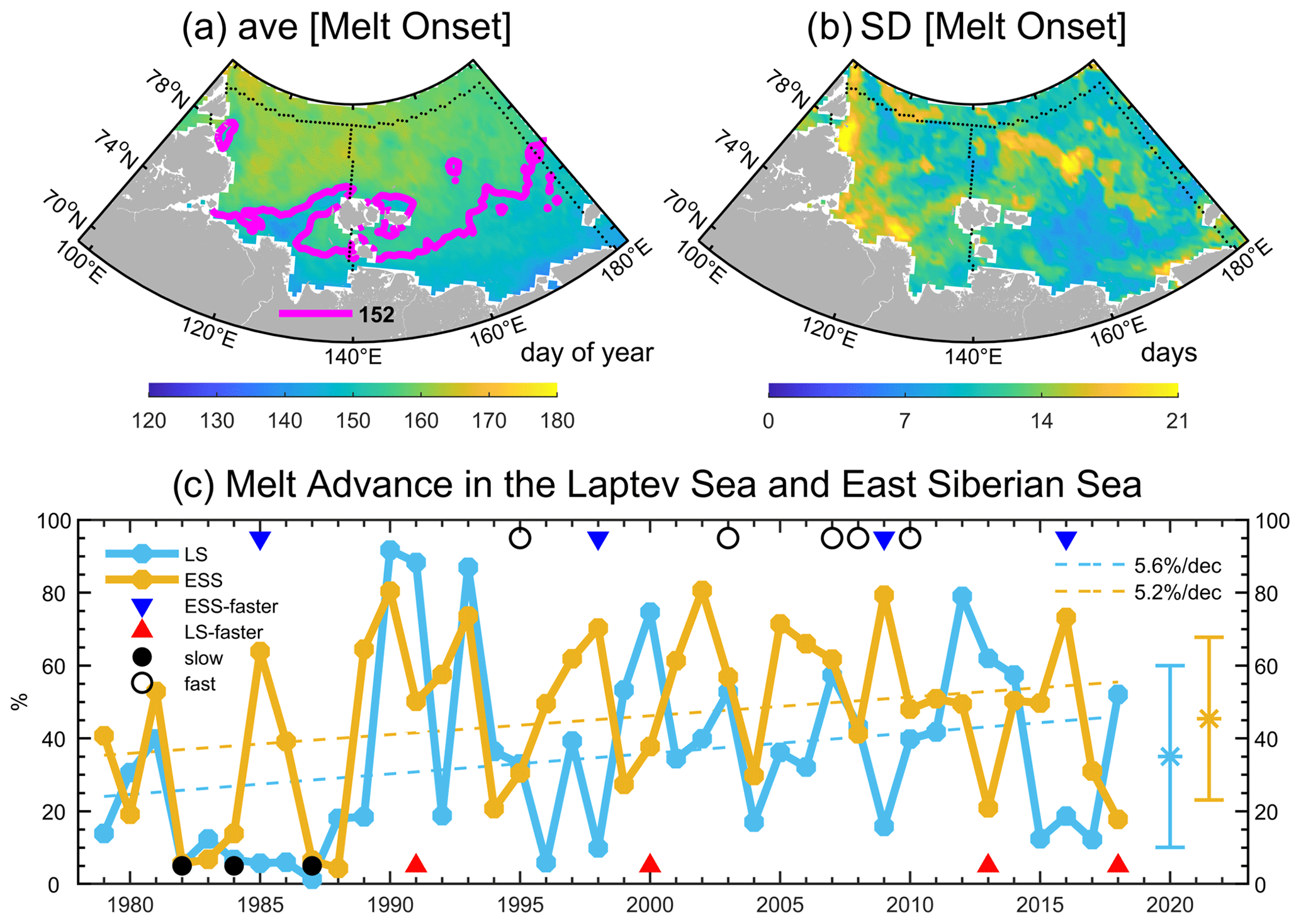
Figure 1 (a, b) Climatology and standard deviation of sea-ice melt onset and (c) melt advance time series in the Laptev Sea and East Siberian Sea, 1979–2018. The magenta lines in panel (a) are the contours of day 152 (day of year), representing the end of May. The areal percentage of sea-ice melt onset earlier than day 152 is defined as melt advance. In panel (c), only the trend in melt advance in the ESS is statistically significant at the 90 % confidence level. The average and standard deviation of the melt advance in the LS and ESS are 35 % ± 25 % and 45 % ± 22 %, respectively. Sample years (16 out of the long time series) that fall into one of four categories are marked (see also Table 1).

Table 1 List of years under different melt advance scenarios.

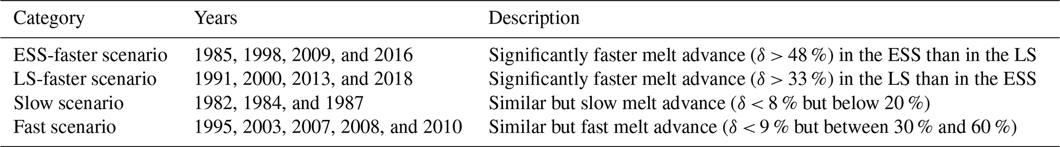
Note: in practical terms, the ESS-faster scenario and LS-faster scenario are selected based on 1 standard deviation of the difference in melt advance between the Laptev Sea and East Siberian Sea. The slow scenario and fast scenario include years when melt advance in the two seas is quite close. All years listed here are marked in Fig. 1c.

Figure 1c shows the time series of MA for the LS and ESS during 1979–2018. The variability is large, ranging from near zero to 100 %. This implies changeable spring conditions on the interannual scale. On average, MA is around 40 % for each sea, meaning that ∼ 40 % of the sea area has experienced sea-ice surface melting at the end of May. In the context of global warming, MA has an increasing tendency in both seas, although this tendency is not quite significant (less than 6 % per decade). This indicates that we sometimes need to pay more attention to the interannual variability than to the long-term linear tendency. We also noticed that relatively slow MA in the 1980s contributes considerably to the overall positive tendency.

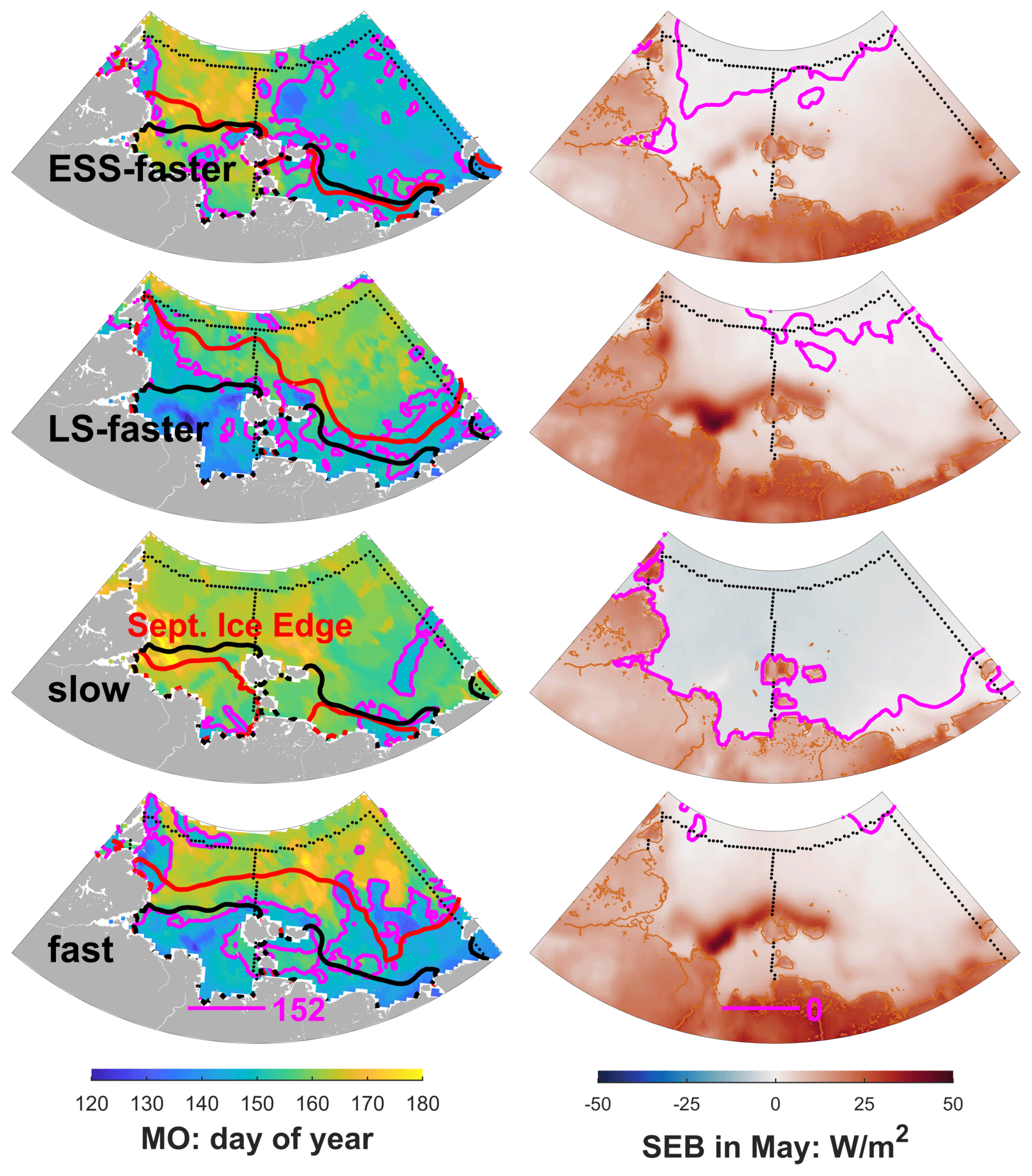
Figure 2 Composites of MO and surface energy balance (SEB) in May for the four scenarios. The left column shows the MO patterns marked by magenta contour lines with the value on day 152 (day of year), which represents the end of May. Red contour lines show the composite September ice edge, while black contour lines denote the climatological September ice edge for 1979–2018. The right column is the SEB in May, with magenta contour lines of zero. Black dots denote the boundaries of the LS and ESS in both columns.

Another feature is related to the relationship of MA between the LS and ESS. In some years, MA in both the LS and ESS is slow, as in the 1980s; in other years, MA in both seas may be fast; and in still other years, MA can be substantially different in the two seas. Thus, four categories of sample years are selected for further composite analysis (Table 1 and markers in Fig. 1c; MA difference between the LS and ESS is shown in Fig. S2), which represent four basic scenarios for MA in this region. Specifically, years with significantly faster MA in the ESS than in the LS (δ > 48 %) are grouped as the ESS-faster scenario, while years with significantly faster MA in the LS than in the ESS (δ > 33 %) are classified as the LS-faster scenario. The slow scenario includes years when MA in both seas is slow (below 20 %), while the fast scenario consists of years when MA in both seas is relatively fast (between 30 % and 60 % at the same time). So, two pairs of contrasting categories are formed (the ESS-faster scenario vs. the LS-faster scenario and the slow scenario vs. the fast scenario). Note that to some extent the latter two scenarios represent the contrast between the 1980s and subsequent decades. Such categorization also reflects the large variability in MA in spring from an interannual perspective.

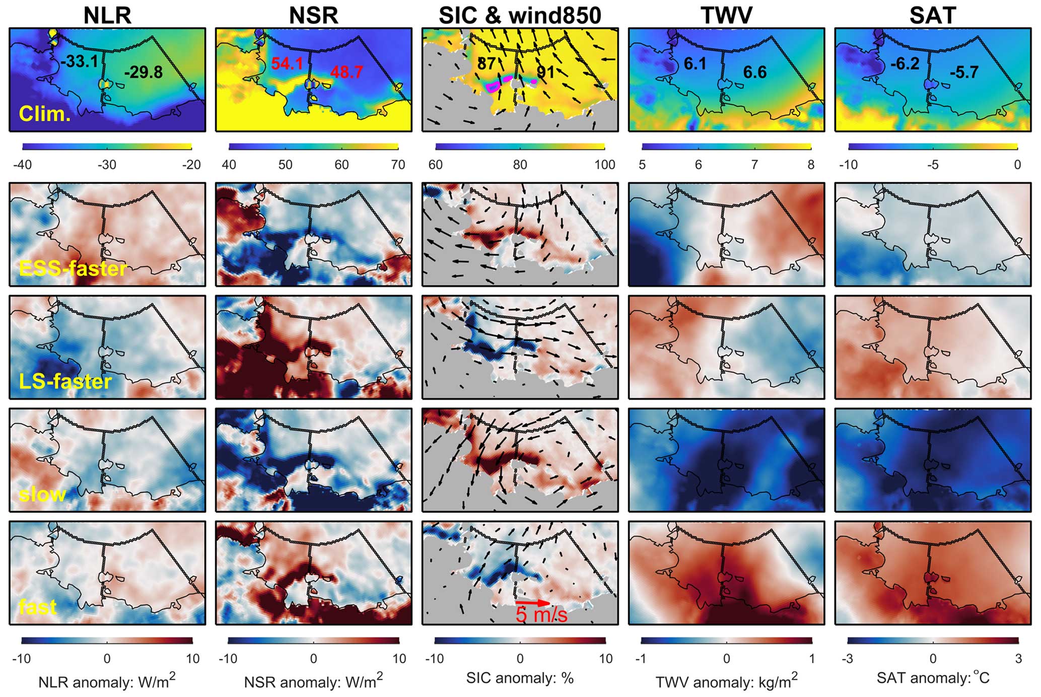
Figure 3 Climatology (first row) and composite anomalies for the four scenarios (lower four rows) of relevant atmospheric and sea-ice variables in May: NLR, NSR, SIC and winds at 850 hPa, TWV, and SAT. Numbers within the LS and ESS are the respective region-mean values. Note that magenta lines in the climatological SIC fields denote contours of 75 % SIC values, which suggest the location of polynyas.

Composite results show that the ESS-faster scenario has substantially earlier MO, i.e., faster MA in the ESS than in the LS, while the LS-faster scenario has a somewhat opposite signal (indicated by the magenta line in Fig. 2). For the slow scenario, little area in either sea has experienced MO until the end of May, indicating slow MA; for the fast scenario, nearly half of both seas has begun to experience sea-ice surface melting, indicating fast MA at almost the same pace. From the surface energy balance (SEB) in May, we find consistent patterns. With the zero lines of SEB as a reference, the ESS-faster scenario has relatively more positive SEB in the ESS than in the LS, while the opposite is true for the LS-faster scenario. For the slow scenario, SEB is negative over most of the two seas, while for the fast scenario, SEB is positive in both seas. This fits well with common sense. Although MA-related albedo changes may amplify the SEB signals in a two-way interaction, it is fair to say that SEB in May drives different patterns of MA (see individual years in Fig. S3).

In the next section, we investigate systematic processes under different MA scenarios that involve the atmosphere, sea ice, and surface energy fluxes.

3.2 Dynamic and thermodynamic processes under different melt advance scenarios

Climatologically, SEB is basically positive (∼ 5 W m⁻²) across the two seas in May (see the first row in Fig. S4). Among the components, it is positive net shortwave radiation (NSR) that compensates for losses from net longwave radiation (NLR), SLHF, and SSHF. This implies that on average the atmosphere receives energy from the surface through the latter three components in May. SAT is around −6 °C, while sea ice almost fully covers the ocean (∼ 90 %; see the first row in Fig. 3). In the lower troposphere (850 hPa), southeasterlies blow across the region, which to some extent explains the existence of polynyas in the middle of LS, i.e., regions where sea-ice concentration is below 75 %. Note that Fig. 3 shows only selected vital variables; other relevant factors can be found in Figs. S4–S7.

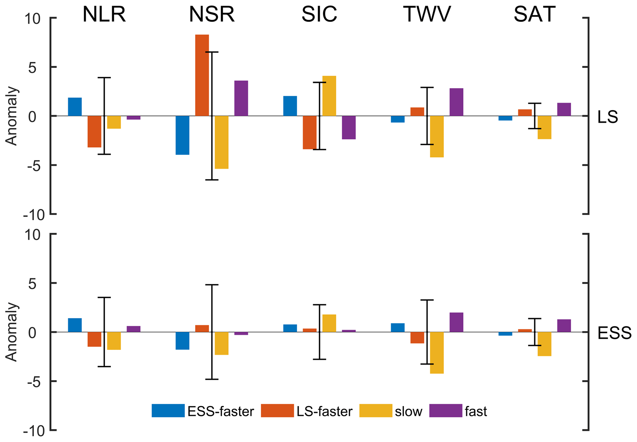
Figure 4 Region-mean composite anomalies in the LS and ESS for the four scenarios shown in Fig. 3. The error bars denote the corresponding standard deviations for 1979–2018. The variables of NLR, NSR, SIC, TWV, and SAT have units of W m⁻², W m⁻², %, kg m⁻², and K, respectively. Here, SIC is represented by the areal percentage of sea-ice cover relative to the whole sea. To facilitate viewing, TWV is scaled by a factor of 5.

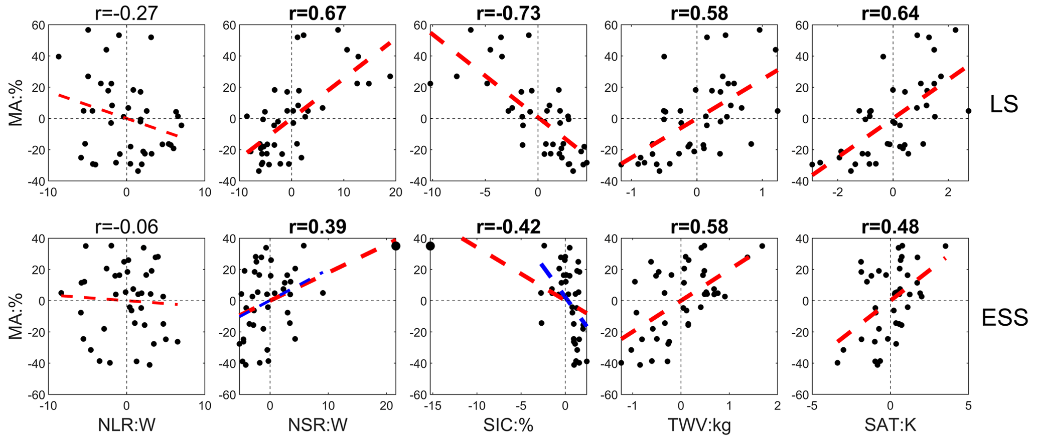
Figure 5 Scatter plots for the period 1979–2018, illustrating the relationship between the melt advance (MA) anomaly and region-mean anomalies of factors shown in Figs. 3 and 4. Thick dashed red lines represent linear fits above the 95 % confidence level. Bold titles represent correlations above the 95 % confidence level. In the second and third panels of the bottom row, thin and thick dashed blue lines denote linear fits after the removal of an outlier, identified by a larger black dot.

In the ESS-faster scenario (see the second row in Fig. 3 and blue bars in Fig. 4), prevailing northeasterlies in the lower troposphere tend to increase SIC and reduce polynya area, especially for the LS, which increases surface albedo and decreases solar radiation absorption. The northeasterlies seem to also bring slightly cool air masses to the region, and slightly moist air masses to the ESS. Given that sea-ice cover is more packed, longwave radiation loss from the surface to the atmosphere is reduced, which to some extent compensates for the reduced solar radiation absorption. Due to the greater negative anomaly of solar radiation absorption in the LS, the net surface energy balance is a loss in the LS but a gain in the ESS (Figs. S4 and S6). In addition, sea-ice surface melting is usually preconditioned by increased water vapor in the atmosphere (Mortin et al., 2016). So, faster melt advance in the ESS is expected as TWV is increased in the ESS. However, in this case, as depicted in Fig. 4, no anomaly extends beyond the interannual standard deviation for the LS and ESS, suggesting a risk of over-interpretation. One plausible explanation is that the normal state in this region tends to resemble the ESS-faster scenario, as indicated by Fig. 1a and the higher climatological melt advance value in the ESS compared to the LS shown in Fig. 1c. Additionally, multiple atmospheric setups may lead to the ESS-faster scenario, highlighting the considerable variability in springtime conditions. Hence, the low signal-to-noise ratio is understandable. It is worth noting that the LS exhibits more notable differences, consistent with its significant polynya activity.

For the LS-faster scenario (see the third row in Fig. 3 and red bars in Fig. 4), wind fields at 850 hPa show unified westerlies over the LS and northwesterlies over the ESS, which to some extent account for the reduced sea-ice cover in the LS and the slightly packed sea ice in the ESS. While the westerlies may not fully account for the reduced sea ice in the LS, this circulation includes an offshore wind component in the western LS, resulting in increased polynya opening. This includes polynyas such as the Northeast Taymyr polynya, the Taymyr polynya, and the Anabar–Lena polynya (Krumpen et al., 2011). So, we see a substantial increase in solar radiation absorption (beyond 1 standard deviation) in the LS. While longwave radiation loss is somehow enhanced, the net surface energy balance is still a gain for the LS and a loss for the ESS. The westerlies may also bring warm and wet air masses from the North Atlantic and contribute to positive anomalies of TWV and SAT in the LS, which promote faster MA. We may expect that reduced sea-ice cover in the LS enables more moisture to be released from the exposed ocean. However, latent heat loss as well as sensible heat loss toward the atmosphere in the LS weakens (Figs. S4 and S6), which suggests that warmer and moister atmosphere is mainly a result of air mass transport and in turn reduces turbulent heat loss from the surface.

For the slow scenario (see the fourth row in Fig. 3 and orange bars in Fig. 4), a cyclonic anomaly in the lower troposphere, which is centered on the ESS, pushes sea ice against the southern coast in the western half of the LS, and against the fast ice zone in the eastern half, thereby preventing polynya formation. More sea-ice cover in both seas decreases solar radiation absorption. Meanwhile, this region is under the influence of cold and dry air masses (beyond 1 standard deviation), which induce a large loss of longwave radiation and SSHF from the surface. As a whole, we see unified surface energy deficits in the LS and ESS (beyond 1 standard deviation). Note that all 3 sample years are from the 1980s. So, the larger sea ice cover and cooler atmosphere mainly reflect the Arctic state in the 1980s, which is a decadal phenomenon rather than an interannual characteristic. We also examine the monthly snowfall under the four scenarios (Fig. S5). For this region, snowfall dominates the total precipitation in May. Especially for the slow melt advance scenario, snowfall is abnormally high, which will also result in high surface albedo.

For the fast scenario with sample years after the 1980s (see the last row in Fig. 3 and purple bars in Fig. 4), southerlies in the lower troposphere blow mainly across the LS, which drive sea ice off the coast, open the polynya, and in turn increase shortwave radiation absorption. At the same time, the southerlies bring warm and wet air masses to this region, which substantially reduce the SSHF loss from the surface. As a result, we see a positive net surface energy balance in this region and relatively fast MA.

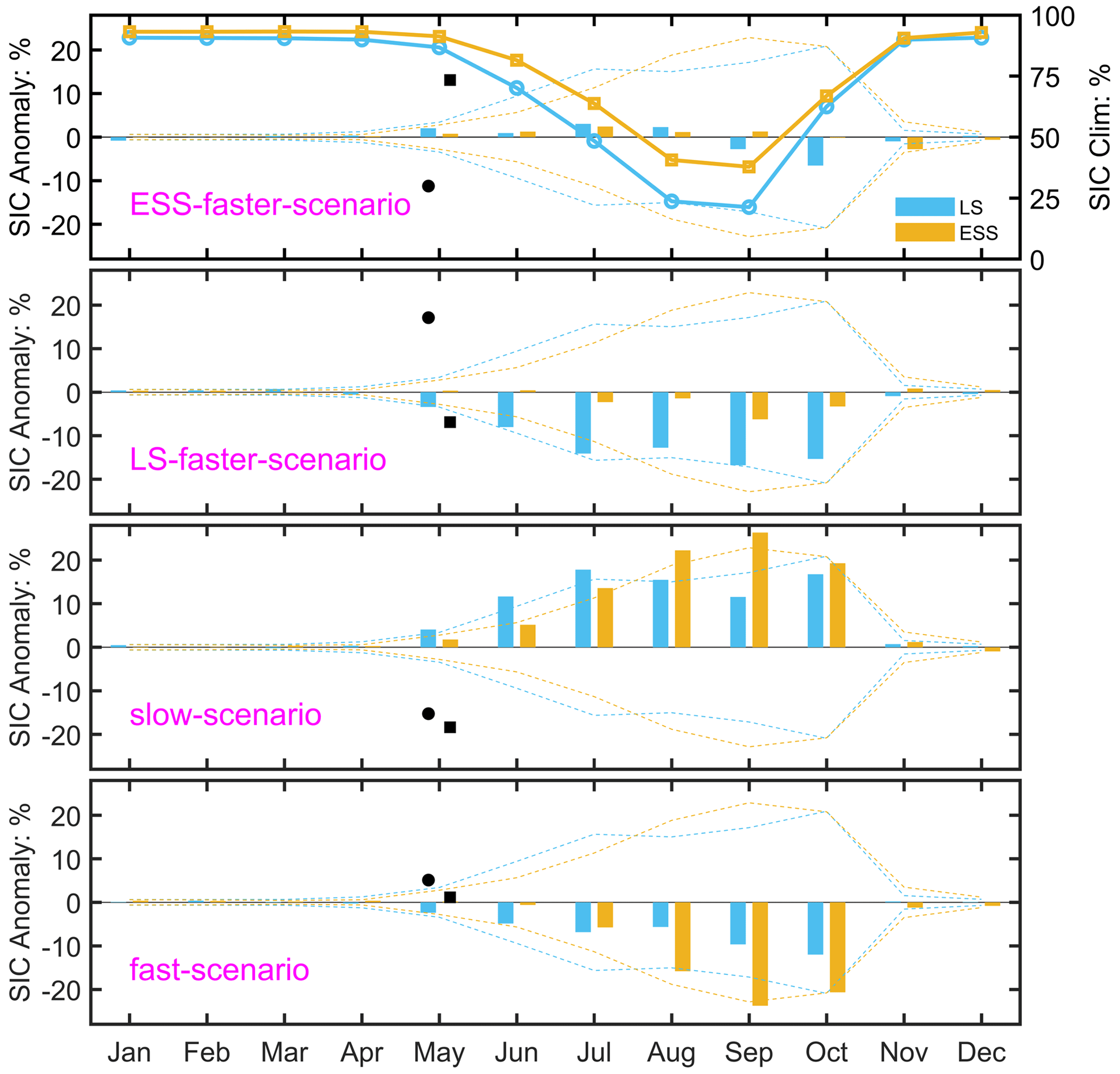
Figure 6 Annual cycle of SIC anomaly in the four scenarios of melt advance. SIC is denoted by the areal percentage of sea-ice cover relative to the whole sea. Dotted lines are the standard deviations. The mean melt advance in the LS and ESS is also marked by solid dots and squares.

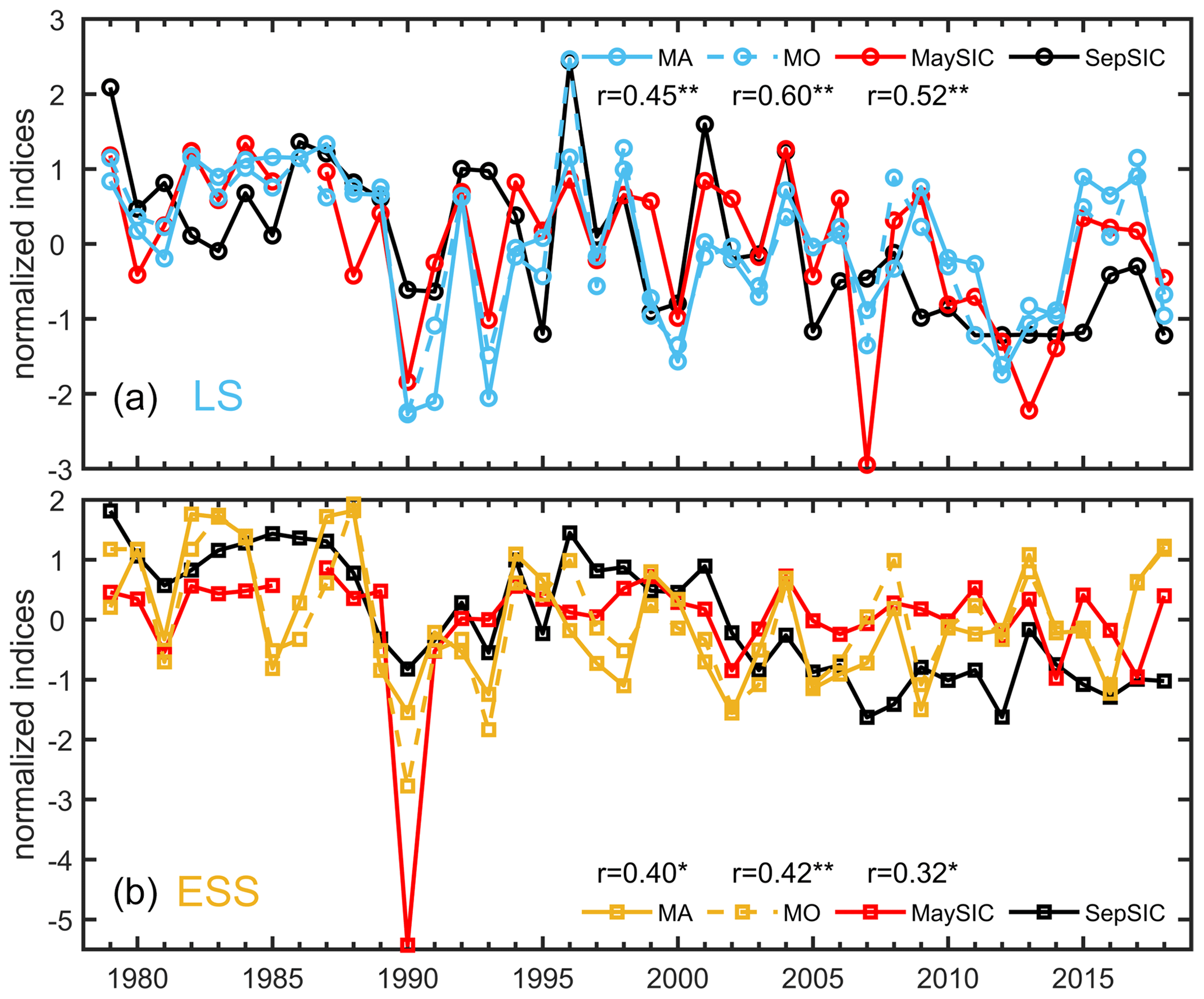
Figure 7 Sea-ice surface melt advance, average melt onset, and sea-ice concentration (SIC) in May and September in the Laptev Sea (a) and East Siberian Sea (b) from 1979 to 2018. The May and September sea-ice cover is denoted by the areal percentage relative to the whole sea. All variables have been normalized. For better visualization, melt advance is multiplied by −1. Correlation coefficients with double asterisks denote 99 % confidence, while those with a single asterisk denote 90 % confidence.

The composite analysis above indicates that circulation in the lower troposphere in spring in this region can be quite changeable (see individual years in Fig. S8), which can have two effects: one is related to sea-ice dynamics and the other involves moisture and air mass advection. The former produces strong regulation of NSR due to albedo changes, while the latter has everything to do with the atmospheric state, which favors sea-ice surface melting when the atmosphere is warm and wet.

Figure 5 further shows the statistical correlation related to MA, covering the years from 1979 to 2018. In general, we see that faster MA is accompanied by warm and wet atmosphere. The related atmospheric circulation in the lower troposphere may also drive reduced SIC and subsequent increased solar radiation absorption. Note that the variability in SIC and NSR in the ESS is smaller than in the LS if the single outlier is removed from the ESS data (see the second and third panels in the bottom row of Fig. 5). Once more, this is related to the significant polynya activity observed in the LS. In addition, Mortin et al. (2016) argued that on a synoptic scale, increased water vapor in the atmosphere favors stronger DLR, which promotes sea-ice surface melting. Such conclusion makes sense when we focus on sea ice and the atmosphere above. While we examine this from the perspective of the whole region, including the effects of the open ocean, results here suggest that on the subseasonal scale, net longwave radiation has little connection to MA (see the first column in Fig. 5). To some extent, the weak correlation even shows that on the monthly scale, longwave radiation loss tends to be more when SEB is more and MA is faster, which suggests some negative feedback probably related to the open ocean.

When NSR is strong, downward shortwave radiation tends to be less (see Fig. S9), which is expected from more moisture in the atmosphere. However, cloud analysis based on ERA5 reanalysis does not suggest significant effects of clouds. Total cloud cover in this region generally is larger than 90 % in May, and the interannual anomaly is relatively small (less than 5 %; see Fig. S5). This indicates that from the perspective of the anomaly, water vapor rather than cloud cover has considerable radiation effects in the springtime. Given the large uncertainty in clouds in current datasets, this remains an open question.

To what extent do different sea-ice surface melting scenarios in spring have implications for sea-ice cover in summer? Could we gain seasonal prediction skill based on the detection of sea-ice surface melting in spring? For the selected melt advance scenarios, sea-ice cover in September responds somewhat accordingly (see the left column in Fig. 2). In the ESS-faster scenario, the sea-ice edge in September is close to the climatology. This echoes the fact that the ESS-faster scenario reflects the climatology of melt advance as well (Fig. 1a). In the LS-faster scenario, sea-ice edge in September retreats more northward in the LS part. In the slow scenario, the sea-ice edge is nearer to the southern coast, while in the fast scenario, the sea-ice edge retreats considerably in both seas. The results above suggest that sea-ice edge in September tends to be northward if melt advance at the end of May is fast. Further investigation of seasonal transition of sea-ice cover in the four melt advance scenarios indicates a similar relationship (Fig. 6).

Figure 7 shows that in both the LS and ESS, melt advance in spring is significantly correlated with sea-ice cover in September, which is consistent with previous studies utilizing melt onset as a predictor of summer sea ice (Petty et al., 2017; Wang et al., 2011). Besides this, it has a similar prediction skill (statistical correlation) as average MO or SIC in May. In general, the connection between springtime and summer seems to be stronger in the LS than in the ESS. Given that the metric of melt advance can be reliably defined on the same day every year (not necessarily the end of May), it has the potential to be fed into the statistical or artificial intelligence prediction of summer sea-ice cover once real-time satellite detection is available. At least, it can be commonly used as the average melt onset. Beyond this, for the prediction of summer sea-ice cover, the seasonal evolution from spring to summer is still a challenge as it is not fully understood.

4 Discussion

In this study, sampling for different scenarios of sea-ice melt advance is based on the melt onset dataset, which is a satellite observation product. To our knowledge, ERA5 to some extent incorporates the sea-ice concentration dataset of OSI SAF but not the melt onset dataset (Hersbach et al., 2020). ERA5 atmospheric reanalysis and different melt advance patterns can be seen as independent sources of information and their consistency should provide more confidence in the results.

In fact, the concept of melt advance can be used for the whole Arctic and can describe how sea-ice surface melting advances in spring. As mentioned above, melt advance can also be used as relatively independent information with reference to an atmospheric-reanalysis dataset. Liang and Zhou (2023) identified three modes of melt onset in the LS and ESS by empirical orthogonal function (EOF) decomposition. The positive L mode and E mode in their study correspond to the LS-faster scenario and ESS-faster scenario, while the positive and negative LE mode relates to the fast scenario and slow scenario, respectively.

Regarding the SIC anomaly in the LS and ESS, we should bear in mind that before melting, the shelf areas of the LS and ESS are covered by extensive fast ice (up to 200 km wide), which is formed by April (Selyuzhenok et al., 2015). SIC in May can increase due to specific wind fields, but it probably does not consolidate against the land. Instead, the SIC anomaly is closely related to polynya development. As Fig. 3 shows, the largest SIC anomaly under the four scenarios usually occurs around the polynya region (Willmes et al., 2011).

5 Conclusions

In this study, the metric of melt advance (MA) is used to measure sea-ice surface melting instead of region-mean melt onset. MA is defined as the areal percentage of a sea in which the sea-ice surface has begun to melt at the end of May, in this case the Laptev Sea (LS) and East Siberian Sea (ESS). This metric has the potential to help seasonally predict summer sea ice for the whole Arctic.

Four representative scenarios of melt advance in the LS and ESS are identified: the ESS-faster scenario, LS-faster scenario, slow scenario, and fast scenario. Composite analyses reveal that in these distinct scenarios of melt advance, atmospheric circulation, sea-ice dynamics (polynya activities), air mass advection, and surface energy fluxes are related to each other. The ESS-faster scenario is associated with a positive TWV anomaly over the ESS and a negative TWV anomaly over the LS. The LS-faster scenario and fast scenario seem to occur when a polynya in the Laptev Sea opens. But the slow scenario mainly reflects the cool Arctic state in the 1980s. In addition, polynya activity in this region and initial sea-ice conditions cannot be neglected either.

Although sea-ice melt advance as well as average melt onset and sea-ice cover in May are both statistically correlated with sea-ice cover in September, seasonal evolution can, to a large extent, disturb this linkage. This study suggests a need to further investigate the changeable spring circulation in the lower troposphere and seasonal evolution in the Arctic.