the Creative Commons Attribution 4.0 License.
the Creative Commons Attribution 4.0 License.
 | 26 Jun 2024
Mapping geodetically inferred Antarctic ice surface height changes into thickness changes: a sensitivity study
Natasha Valencic
Linda Pan
Konstantin Latychev
Natalya Gomez
Evelyn Powell
Jerry X. Mitrovica
Determining recent Antarctic ice volume changes from satellite altimeter measurements of ice surface height requires a correction for contemporaneous vertical crustal deformation. This correction must consider two main sources of crustal deformation: (1) ongoing glacial isostatic adjustment (GIA), that is, the deformational, gravitational, and rotational response to Late Pleistocene and Holocene ice and ocean mass changes and (2) modern ice mass change. In this study, we seek to quantify the uncertainties associated with each of these corrections. Corrections of ice surface height changes for correction 1 have generally involved the adoption of global models of GIA defined by some preferred combination of ice history and mantle viscoelastic structure. We have computed the GIA correction generated from a coupled ice sheet–sea level model and a realistic Earth model incorporating three-dimensional viscoelastic structure. Integrating the difference between this correction and those from recent GIA analyses widely adopted in the literature yields an uncertainty in total present-day ice volume change equivalent to approximately 10 % of Antarctic ice mass loss inferred for the period 2010–2020. This reinforces earlier work indicating that ice histories characterized by relatively high excess ice volume at the Last Glacial Maximum may be introducing a significant error in estimates of modern melt rates. Regarding correction 2, a spatially invariant scaling has commonly been used to convert GIA-corrected ice surface height changes obtained from satellite altimetry to ice volume estimates. We adopt modeling results based on a projection of Antarctic ice mass change over the period 2015–2055 to demonstrate a spatial variability in the scaling of up to 10 % across the ice sheet. Furthermore, using these calculations, we find a systematic error of ∼ 3 % in the projected net ice volume change, with most of the difference arising in areas of West Antarctica above mantle zones of low viscosity.
- Article
(4262 KB) - Full-text XML
- BibTeX
- EndNote


Modern satellite measurements of ice volume are critical to estimates of global sea level change. Geodetic systems, such as the Geoscience Laser Altimetry System aboard the Ice, Cloud, and Land Elevation Satellite (ICESat), measure changes in the height of the ice surface over time. To convert these measurements of surface elevation change (henceforth referred to as ice surface height change) into estimates of ice mass change, several corrections must be applied. A “firn correction” is necessary, which is based on information regarding the density and thickness of ice–firn layers. Corrections are also required for crustal elevation changes due to both glacial isostatic adjustment (GIA) and the viscoelastic response of the solid Earth to modern-day melt (Groh et al., 2012).
GIA represents the ongoing deformational, gravitational, and rotational response of the Earth to mass transfer between the cryosphere and the open ocean across the Pleistocene glacial cycles and into the Holocene (Mitrovica and Milne, 2002). Model-based corrections of altimeter data for GIA require constraints on ice history and mantle viscoelastic structure. Uncertainties in either of these will propagate forward and result in uncertainties in estimates of ice thickness change. Ice histories are commonly inferred by fitting GIA models to sea level datasets in both the near field and far field of ice sheets (Lambeck et al., 2014; Peltier et al., 2015). Ice sheet modeling, either in combination with GIA modeling or as a standalone approach, can also be used to constrain ice history (Whitehouse et al., 2012; Gomez et al., 2013, 2018). Mantle viscosity fields have been implemented in GIA modeling at various levels of complexity, from one-dimensional models with as few as three layers to full three-dimensional variability. One-dimensional models assume that the viscosity of the mantle depends only on depth (Lambeck et al., 2014; Peltier et al., 2015), while their more computationally expensive three-dimensional counterparts include lateral variation in the mantle viscosity (Li et al., 2020). This complexity is advisable when modeling GIA in the Antarctic region due to large variations in lithospheric thickness and viscosity beneath the continent. Notably, the mantle beneath parts of West Antarctica is several orders of magnitude less viscous than under East Antarctica (Powell et al., 2020) and lithospheric thickness increases by as much as a factor of ∼ 4 from West to East Antarctica.
Correcting altimeter data for crustal deformation – i.e., mapping altimeter observations of ice surface height changes into ice thickness changes – due to modern-day melting is generally based on elastic one-dimensional Earth models. In this case, the elastic Love number theory (Farrell, 1972) has been applied to approximate the ratio of ice thickness to ice surface height changes. In previous work, this ratio, which we denote by α, was fixed at a value of α=1.0205 by considering the average spatial scale of various Antarctic drainage basins (Groh et al., 2012). That is, the field of firn- and GIA-corrected ice surface height change was multiplied by this constant to estimate ice thickness change. Subsequent studies of Antarctic ice elevation measurements have applied the scale factor used in the Groh et al. (2012) paper as a correction in the conversion of ice surface height changes to ice mass changes. For instance, in Schröder et al. (2019), a study using 4 decades of altimetry data from multiple satellite missions, surface elevation changes are multiplied by a value of α=1.0205 to account for elastic solid Earth rebound effects. The use of this ratio is not restricted to Antarctica; in Kappelsberger et al. (2021), the same α=1.0205 is applied to surface elevation changes in northeast Greenland. However, the full expression for the mapping derived from the Love number theory indicates the ratio is dependent on spatial scale and will thus be geographically variable. Furthermore, the adoption of a constant scaling neglects both crustal deformation due to ocean loading and viscous effects (see Sect. 2 for full details). Given the low mantle viscosity below parts of Antarctica, viscous effects may impact the relationship between ice surface height and thickness changes over timescales of a few decades, and thus the use of purely elastic models may introduce an error even over such short timescales (Powell et al., 2020).
In this article, we seek to quantify the level of uncertainty in ice volume estimates derived from altimetry data introduced by uncertainties in the treatment of GIA and crustal deformation due to modern melting. The next section summarizes the Love-number-based mapping between ice surface height and ice thickness changes. The Results section has two parts. First, we use published models to quantify the range of GIA corrections for ongoing crustal uplift in Antarctica. Next, we generate a crustal uplift field from a published projection of Antarctic ice evolution in the 21st century and use this field as a synthetic dataset to explore the geographically variable mapping between ice surface height and ice thickness changes in response to modern ice mass change.
We begin with the spherical harmonic formulation of the sea level equation on a one-dimensional elastic Earth. The global sea level change at colatitude θ and east longitude ϕ, ΔSL(θ,ϕ), is given by Kendall et al. (2005) as
where a and Me are the radius and mass of the Earth and ρi and ρw are the densities of ice and water. ΔI and ΔS are the spherical harmonic coefficients of degree ℓ and order m of ice thickness change and ocean height change, respectively. These are associated with the basis function Yℓm, which is normalized in our calculations so that
where the asterisk denotes complex conjugation. Furthermore, the following applies:
In the latter equation, kℓ and hℓ are elastic Love numbers that govern perturbations in the gravitational potential and crustal elevation, respectively. The unity term in the definition of Eℓ represents the direct gravitational potential perturbation due to load redistribution. The global sea level change is given by the difference in perturbations to the sea surface and crustal elevations. The latter can be isolated from Eq. (1) to obtain
One can write an expression for the spherical harmonic coefficients of ice surface height change as a simple sum of the coefficients of ΔR and ΔI:
which allows us to express the change in ice thickness ΔI as
Using Eq. (4), we can write
Solving for the change in ice thickness gives the following final expression:
This expression relates ice thickness changes to ice surface height (or surface elevation) changes (ΔH) and ocean thickness changes (ΔS) and makes two assumptions. First, that viscous effects can be ignored and, second, that elastic Earth structure varies with depth alone. The latter introduces negligible error (Mitrovica et al., 2011). In applying this expression to regions proximal to ice cover, it is common to neglect ocean load changes since they are relatively small. Neglecting this term gives
Thus, we have the following:
The same expression was derived by Groh et al. (2012) although their derivation was based on considering the gravitational effects of ice mass changes and crustal uplift, following results in Wahr et al. (1998). The expression indicates that the mapping between ice surface height and ice thickness changes is dependent on spatial scale (via the spherical harmonic degree ℓ), as shown in Fig. 1.
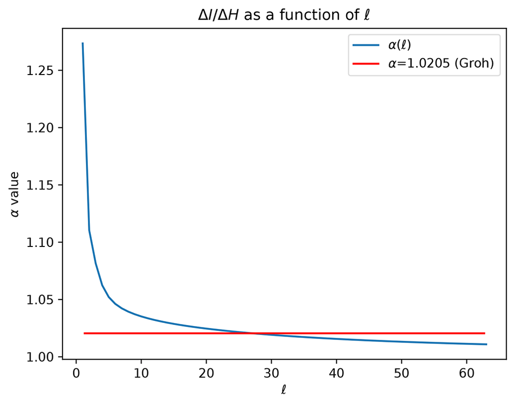
Figure 1The value of the parameter αℓ as a function of the spherical harmonic degree ℓ, as defined in Eq. (10). The red line indicates the value of αℓ adopted in Groh et al. (2012).
As noted, Eqs. (9) and (10) assume that the response of the solid Earth to modern ice loss in the Antarctic region can be represented by an elastic Earth model. The inaccuracy this introduces will be a function of the timescale of ice loading that is considered and the viscosity of the underlying mantle. In the Results section, we investigate this issue by considering both elastic and viscoelastic Earth models. Our predictions also include the impact of water height changes, ΔSℓm, on the mapping. Although Groh et al. (2012) derived Eq. (10), they assumed that the second term in brackets in these equations could be replaced a simple constant (0.0205) that they computed by considering the value that this second term would take on if one used a spatial scale consistent with the mean scale of Antarctic drainage basins. Their assumption, in this case that α=1.0205 (red line in Fig. 1), removes the dependence of α on spatial scale.
In all the calculations presented below, we adopt a specified ice-load history and compute gravitationally self-consistent sea level variations using a Maxwell viscoelastic Earth model. The sea level theory accounts for migration of shorelines and the feedback of Earth's rotation changes into the sea level (Kendall et al., 2005). The solutions are based on a finite-volume formulation of the surface loading problem which allows for arbitrary, three-dimensional variations in mantle viscoelastic structure (Latychev et al., 2005). The GIA and modern ice mass change calculations are distinguished by the input ice histories, each of which we discuss in turn.
3.1 Glacial isostatic adjustment
The GIA simulations adopt three different ice histories: the global ICE-6G_C model of Peltier et al. (2015), an updated version (Erik Ivins, personal communication, 2023) of the Antarctic model of Ivins and James (2005) (referred to as IJ05), and an ice history derived by coupling a three-dimensional Antarctic Ice Sheet (AIS) model with a GIA-based sea level model (hereafter the G18 model) (Gomez et al., 2018). The G18 model is combined with the non-Antarctic components of the global ICE-5G model (Peltier, 2004), while the non-Antarctic components of the ICE-6G_C model are used to create a global model with the IJ05 Antarctic history. Each of these ice histories is coupled with a viscoelastic Earth model. The ICE-6G_C model is paired with the one-dimensional, three-layer VM5a model, in which the viscosity varies from 5×10²⁰ Pa s in the upper mantle to 3×10²¹ Pa s in the deep mantle (Peltier et al., 2015). The VM5a model has an elastic lithospheric thickness of 90 km. The three-layer IJ05 model includes a lithospheric thickness of 90 km and mantle viscosities of 4×10²⁰ Pa s for the upper mantle, 6×10²¹ Pa s for the lower mantle between 670 and 1200 km depth, and 8×10²² Pa s for the lower mantle between 1200 km depth and the core–mantle boundary (Ivins and James, 2005). The G18 model adopts a three-dimensional Earth model derived by Hay et al. (2017) on the basis of seismic tomographic results (An et al., 2015; Heeszel et al., 2016). This Earth model (H17) has a spatial resolution of 6 km near the surface to 25 km above the core–mantle boundary. The model has a mean lithospheric thickness of 65 km in West Antarctica and 200 km in East Antarctica (Hay et al., 2017). The viscosity beneath West Antarctica reaches values as low as 1018 Pa s (see Fig. 2), consistent with the tectonic rift setting of the region (Wörner, 1999). The elastic structure for all three models is given by the seismic model Preliminary reference Earth model (PREM; Dziewonski and Anderson, 1981). Note that while we computed present-day uplift rates from the IJ05 and G18 models, we obtained these rates for ICE-6G_C directly from the website of the model's creator.
3.2 Modern mass change
Our calculations of the Earth’s response to modern mass change adopt, on input, the fETISH32 (EXP A1) projections to 2055 CE of the Antarctic Ice Sheet (Pattyn, 2017). The projection is one of ∼ 180 such projections included in the Ice Sheet Model Intercomparison Project for CMIP6 (ISMIP6) and is characterized by a net global mean sea level rise of 14.7 cm from 2015 to 2055 (the highest GMSL – global mean sea level – rise in any projection in ISMIP6). We pair this ice projection with three Earth models: a purely elastic Earth model based on PREM and two three-dimensional viscoelastic models, one derived by Austermann et al. (2021) based on results from Richards et al. (2020) (henceforth the RH20 model) and the model adopted in the G18 simulation mentioned above (Hay et al., 2017). The Richards et al. (2020) model is constrained by seismic tomography (Schaeffer and Lebedev, 2014), laboratory measurements of mantle materials, and seismic attenuation measurements. It is characterized by a shallow mantle viscosity of ∼1019 Pa s below West Antarctica (see Fig. 2).
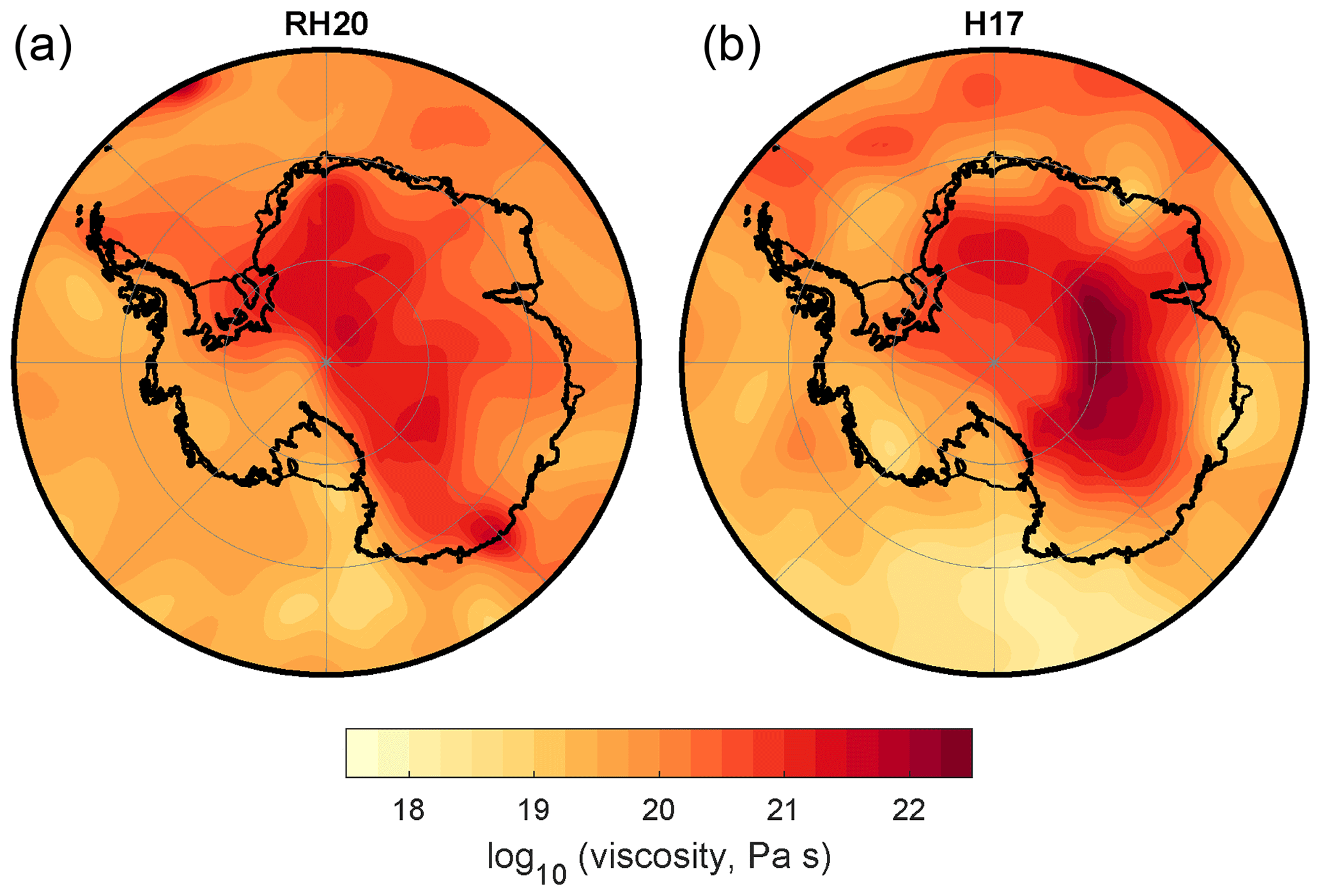
Figure 2Mean viscosities from the base of the lithosphere to 400 km depth under Antarctica in the two three-dimensional viscoelastic Earth models: (a) from Richards et al. (2020) and (b) from Hay et al. (2017). Both models are adopted in the calculation of the Earth's response to modern mass flux, while the latter is also considered in the GIA calculations presented herein.
4.1 GIA correction to altimeter records
Figure 3 shows present-day rates of crustal uplift due to GIA for each ice model paired with its own Earth model: G18, ICE-6G_C, and IJ05. The relative magnitude of the signals is roughly consistent with the excess Antarctic ice volume at LGM, as prescribed in each published model: 6, 10, and 14 m in units of equivalent GMSL for the G18, IJ05, and ICE-6G_C simulations, respectively (Gomez et al., 2018; Ivins and James, 2005; Peltier et al., 2015). Some of the differences may arise from differing levels of ice mass change in the late Holocene across models; however, these variations should be small. In the G18 model, the largest rates of uplift are in Oates Land in East Antarctica, where uplift exceeds 10 mm yr−1 in a small area), and south of the Ronne Ice Shelf (peak rates of ∼ 6 mm yr−1). The ICE-6G_C model predicts uplift south of the Ronne Ice Shelf and in Marie Byrd Land, with rates peaking at about 13 mm yr−1. The IJ05 model locates its highest uplift rates west of the Ronne Ice Shelf and in Marie Byrd Land, where the rates do not exceed 7 mm yr−1.
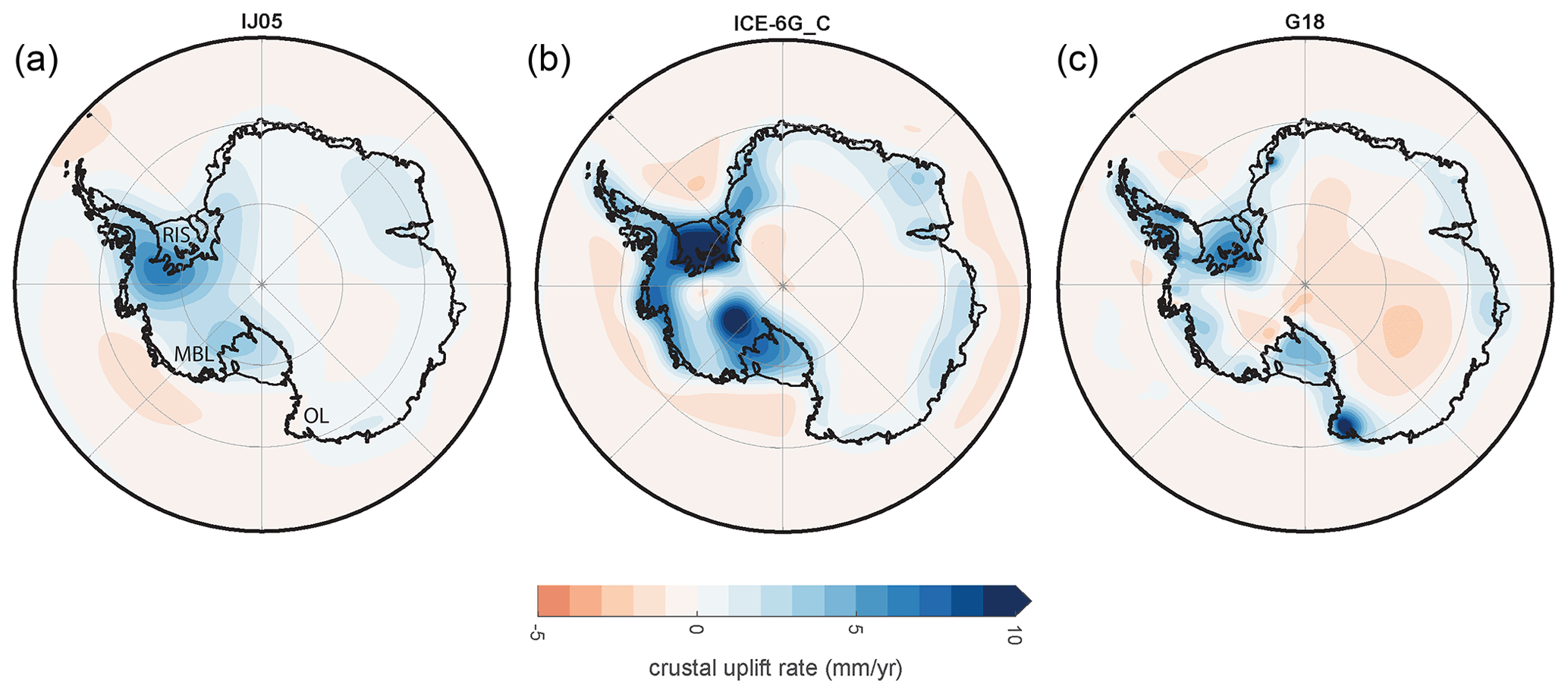
Figure 3Present-day crustal deformation rates due to GIA computed for three different ice history/Earth model combinations: (a) the IJ05 model from Ivins and James (2005), (b) the ICE-6G_C model from Peltier et al. (2015), and (c) the G18 model from Gomez et al. (2018). Areas mentioned in the text are labeled in panel (a) as follows: RIS stands for Ronne Ice Shelf, MBL for Marie Byrd Land, and OL for Oates Land.
The difference maps in Fig. 4 indicate that the GIA correction and therefore the modern ice thickness changes inferred from the residual (GIA-corrected) uplift signal are subject to significant uncertainty. We assume that the G18 model, derived from a GIA calculation based on a more realistic, three-dimensional Earth model and consistent with ice sheet physics, provides the most accurate prediction of uplift rates. The differences in uplift rates in Fig. 4 then represent a reasonable proxy for this uncertainty (though we are not using this term in a rigorous statistical sense) given that the ratio of uplift rate to ice thickness change is close to 1 for the case of modern ice mass change (see below). These differences, when integrated over all present-day Antarctic grounded ice, yield a total ice volume change uncertainty equivalent to 0.028 mm yr−1 global mean sea level change for the IJ05 case and 0.046 mm yr−1 for the ICE-6G_C case. Moreover, these uncertainties would total 1.12 and 1.84 mm over the period 2015–2055.
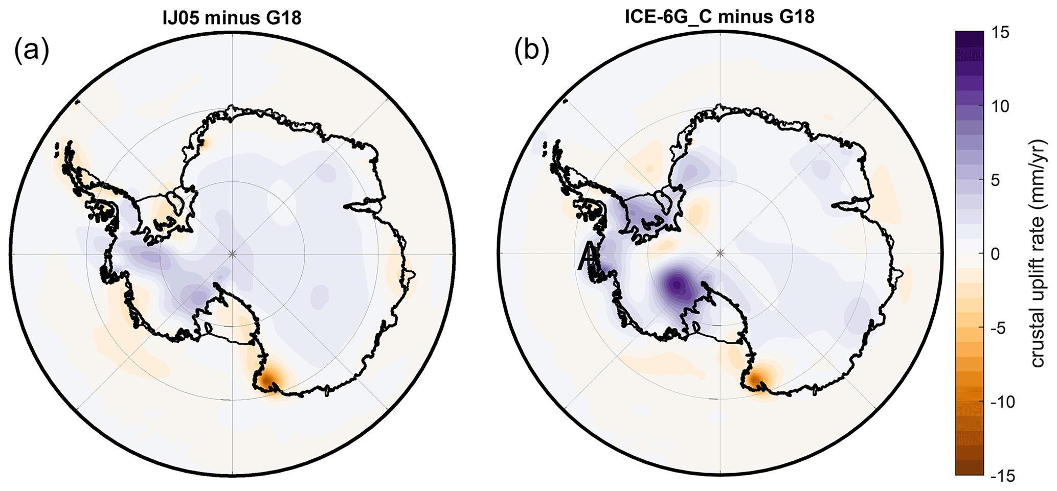
Figure 4Differences in predicted crustal deformation rates between the G18 model and the IJ05 (a) and ICE-6G_C (b) models.
To end this section, we augment the GIA calculation to consider the ongoing impact of Antarctic ice mass changes over the past century. We constructed the ice model by first adopting the ice history from 2003–2015 of Schröder et al. (2019). This loading history has a 10 km spatial resolution and a melt geometry largely focused on the Amundsen Sea Embayment region. To extend the loading history back into the 20th century, we follow the method described in Barletta et al. (2018). We computed the average ice thickness change per year of the Schröder et al. (2019) ice model, scaled it by 25 %, and applied it across the period 1900–2003. This history yields a total GMSL rise of 10.8 mm. The mean crustal displacement rate over the period 2015–2055 computed using the three-dimensional viscoelastic Earth model is shown in Fig. 5. The integral of this field over the Antarctic maps into a correction to any altimeter-derived estimate of ice volume change from 2015–2055 equivalent to 0.32 mm (0.008 mm yr−1) of the global mean sea level.
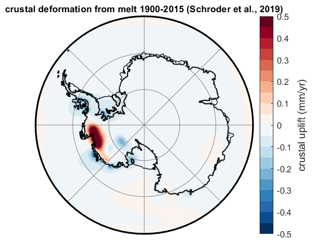
Figure 5The average crustal deformation rate for 2015–2055 due to a melt model from 1900–2015 constructed based on Schröder et al. (2019).
4.2 Mapping altimeter measurements of ice surface height changes to thickness changes
As shown in the theory section (Sect. 2), the mapping between ice surface height and ice thickness changes, αℓ, must be dependent on spatial scale but is commonly approximated as a single scale factor (Groh et al., 2012). To explore the inaccuracy introduced by this assumption, we computed the response of a set of Earth models to the fETISH32 (EXP A1) projection of ice thickness change over the 40 years between 2015 and 2055 (Fig. 6). The computed ratio between ice thickness and ice surface height changes in the case of an elastic Earth model and two three-dimensional viscoelastic models – RH20 (Richards et al., 2020) and the Earth model adopted in the G18 simulation described above (Fig. 2) – is shown in Fig. 7. A cutoff of 10 m of ice surface height change is introduced to focus on the areas of sizable ice mass change. We justify this cutoff by noting that the regions with at least 10 m of ice surface height change are the source of 90 % of the total Antarctic contribution to GMSL rise in the fETISH32 (EXP A1) projection. Since the results in this study are expressed in terms of differences in GMSL rise predictions, it is appropriate to focus on the value of α in regions with sizable contributions to that rise.
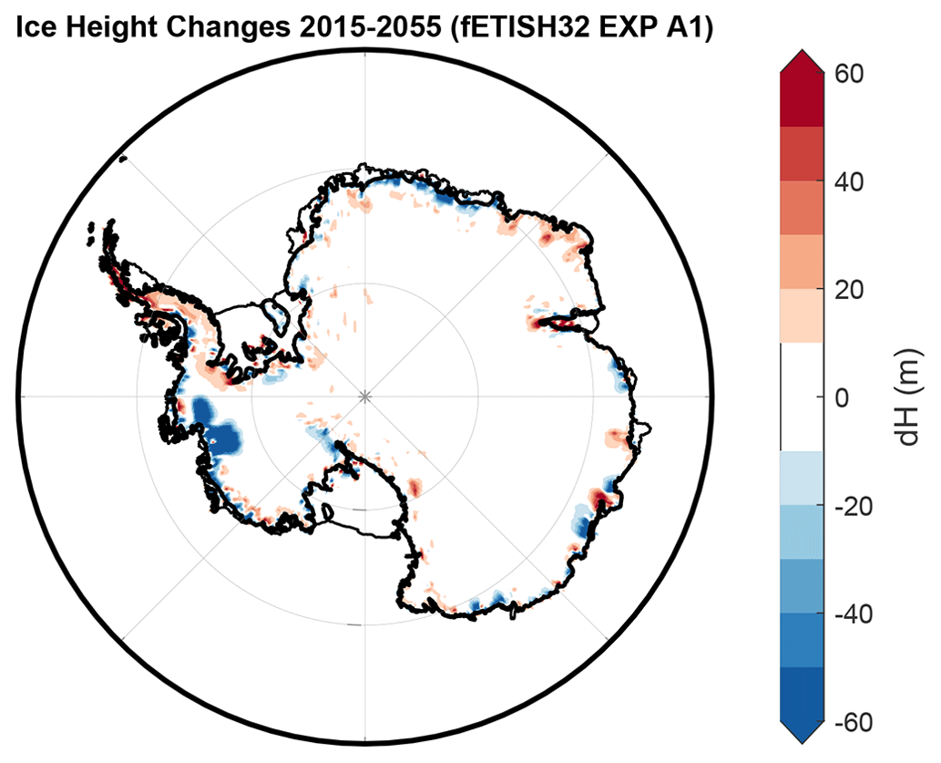
Figure 6Ice thickness change (meters) 2015–2055 CE from fETISH32 (EXP A1).
The value of α varies between 0.98 and 1.07 in areas of the Antarctic with at least 10 m of ice surface height change. The largest variations in this scaling factor from the value of α=1.0205 occur in regions of high mass change, such as Pine Island and Thwaites glaciers. In these two areas, the value of α increases as one moves inland from the coast.
The introduction of viscous deformation has negligible impact over East Antarctica and parts of West Antarctica that are characterized by relatively high viscosity (Fig. 2). The largest impact of viscous effects is once again in the areas of greatest mass flux, near Pine Island and Thwaites glaciers, which overlay regions of relatively low mantle viscosity and where the ratio αℓ grows more quickly relative to the elastic case as one moves inland. This trend becomes more pronounced as the shallow viscosity of the underlying Earth model decreases, as it does in these areas as one moves from considering the RH20 model results to the G18 model results.
Using these projections, we can estimate the error in estimates of total ice volume changes that is incurred by assuming the constant value of α=1.0205. In the case of the projection based on the RH20 viscoelastic model, applying this assumption would underestimate the ice volume loss in the next 40 years by 50, 700, and 400 km3 in the Antarctic Peninsula, West Antarctica, and East Antarctica, respectively. The analogous values are 30, 1200, and 400 km3 for the G18 model. Summing each triplet yields an underestimate of 3.2 and 4.5 mm in units of equivalent GMSL change, respectively, for the RH20 and G18 model projections.
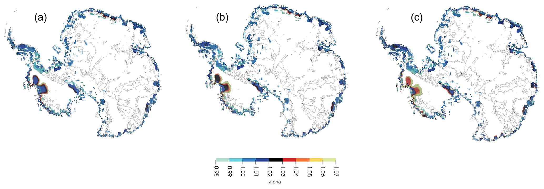
Figure 7The ratio of ice thickness to ice surface height changes (α) from 2015 to 2055 in regions with an ice thickness change greater than 10 m. In panel (a) is a map computed by assuming a fully elastic Earth model. In panels (b) and (c) are the corresponding maps based on the Richards et al. (2020) (RH20) and the Hay et al. (2017) (G18) viscoelastic models, respectively. The gray lines indicate the zero-elevation crustal contour.
To explore the time history of the spatial variation in α, Fig. 8 shows the variation of this ratio, as well as total ice thickness change, in 10-year intervals along a profile through the Amundsen Sea sector of the Antarctic Ice Sheet computed using the H17 viscoelastic Earth model. (The choppiness of the profiles reflects the ∼ 20 km spatial grid of fETISH32 EXP A1 ice history). A trend in the profiles is apparent in the first 30 years, but this trend reverses by the end of the simulation. The value of α comes closest to 1.0205 in the vicinity of the largest ice thickness change but systematically diverges from this number moving away from this location in areas of significant ice mass change.
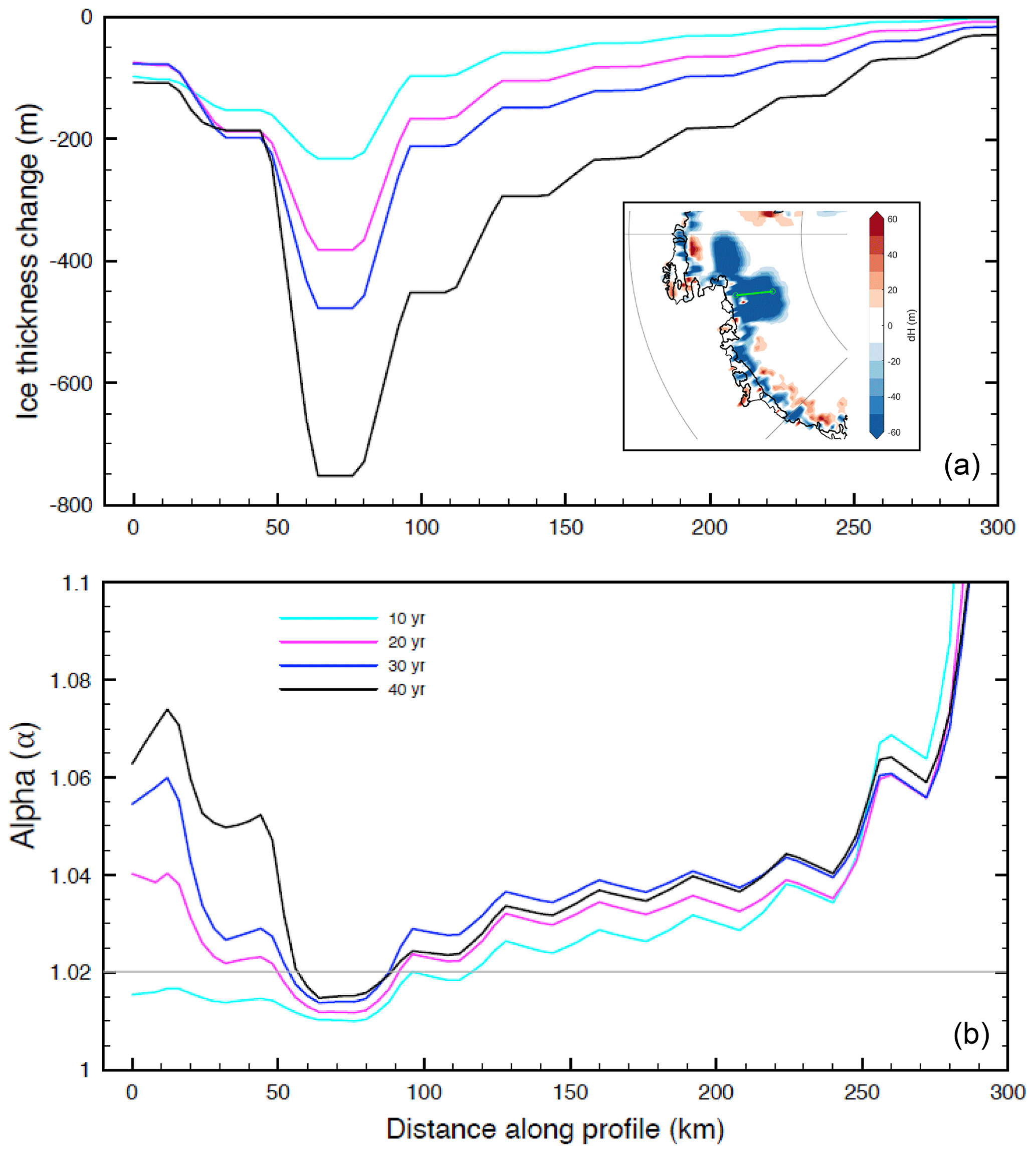
Figure 8The temporal evolution of α in 10-year increments along a profile through the Thwaites Glacier, indicated by the green line in the inset. The distance along the profile is measured from the northern end of the cross section.
Shepherd et al. (2012) noted that significant uncertainty in the GIA correction to Antarctic ice mass change estimates is introduced by uncertainty in the excess volume of Antarctic glaciation at LGM. Their analysis adopted the ice history of Whitehouse et al. (2012), which had an excess ice volume significantly smaller than some previous estimates (8 m in units of equivalent GMSL rise). This ice history was paired with a viscosity profile with a preferred range of upper mantle viscosity of 0.8×10²¹–2.0×10²¹ Pa s. The present analysis has reconsidered this issue using an ice history generated from a coupled ice sheet–sea level model and a significantly more realistic viscoelastic mantle model for the region (i.e., the G18 simulation). The latter is characterized by significant variability in viscosity, including low-viscosity zones beneath some sections of the West Antarctic. We find that the differences in the GIA correction between the G18 model and Earth model–ice history pairs inferred in a recent GIA analysis, when integrated over the Antarctic, map into an uncertainty in total present-day ice volume change of 0.046 mm yr−1 GMSL equivalent for the ICE-6G_C case and 0.028 mm yr−1 for the IJ05 case. These uncertainties are 12 % and 7 %, respectively, of the estimated AIS mass loss over the decade 2010–2020 (Velicogna et al., 2020). Moreover, these differences would represent uncertainties of 1.12 and 1.84 mm GMSL equivalent in altimeter-based estimates of Antarctic ice volume changes from 2015–2055. Neglecting the impact of ice mass change from 1900–2015 would introduce an additional uncertainty of ∼ 0.3 mm GMSL equivalent to altimeter-based estimates of the mass balance from 2015–2055. The significance of these projected uncertainties, which sum to ∼ 2 mm, will, of course, depend on the realized mass flux over this 40-year period.
Previous studies have scaled GIA-corrected altimeter measurements of ice surface height changes into thickness changes using single scaling close to 1.02 (Groh et al., 2012; Schröder et al., 2019; Kappelsberger et al., 2021). The true scaling will depend on both the spatial scale of the loading and also on the rheological properties of the underlying crust and mantle. We have found, using calculations based on a projection of Antarctic mass flux over the next 40 years, that this scaling can vary by ∼ 10 %, i.e., from 0.98 to 1.07, as one moves inland from the coast. There are two reasons for this geographic trend in the error. First, the crustal response at a given site is proportional to the distance-weighted integral of the total load change near that site. Since the change in the ocean load is small close to the coastline relative to the local ice mass change, the integrated load change a site will experience will tend to increase moving inland (i.e., in contrast to a coastal site, an inland site has ice mass change on all sides). Second, the spatial scale of ice streams varies with location: the catchment basin tends to narrow as one moves toward the coastline. As indicated in Fig. 1, the value of α will be smaller when the characteristic scale of the mass change (here, the scale of the catchment basin) decreases.
The error incurred in estimates of ice volume changes based on this constant scaling, when considering the fETISH 32 (EXP A1) projection of modern Antarctic melt from 2015–2055, is ∼ 3 % (4 mm GMSL equivalent relative to the total flux of 14.7 cm GMSL). To reduce this systematic error, we advocate performing a spherical harmonic decomposition of the altimeter-derived ice surface height and scaling the harmonics using the αℓ filter (Fig. 7) to estimate ice thickness changes. While this approach ignores both viscous effects and ocean loading on the isostatic adjustment, we have found that it reduces errors in the estimate of ice thickness changes relative to assuming that α=1.0205. As an example, Fig. 9 shows a map of the error in the estimated ice thickness change over the next 40 years in the vicinity of the Amundsen Sea when ice surface height changes computed using the H17 viscoelastic Earth model are scaled using the αℓ filter. The peak error of 6.2 m is less than 1 % of the peak ice thickness change of ∼ 830 m. Moreover, the RMS error in the αℓ case is a factor of 2.3 times smaller than the error incurred in adopting the assumption of a constant α=1.0205.
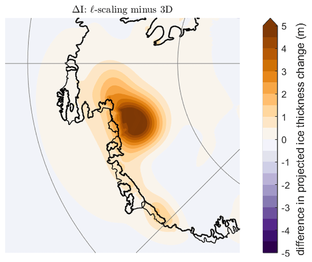
Figure 9The difference between the ice thickness changes predicted by scaling the ice height changes with an ℓ-dependent method and those predicted by a full three-dimensional viscoelastic model.
We have investigated potential errors in estimates of ice thickness change inferred from satellite altimetry measurements arising from (1) errors in the correction for GIA and (2) the mapping of GIA-corrected ice surface height changes to ice thickness changes associated with modern melt using a single (i.e., geographically invariant) scalar. The integrated difference in the present-day uplift across different GIA models amounts to 1–2 mm GMSL equivalent over the next 40 years, while neglecting the impact of ice mass change since 1900 introduces an additional uncertainty of 0.3 mm GMSL equivalent. The use of a spatially invariant scalar to map ice height changes to ice thickness changes results in a systematic underestimate of ice mass change when compared to values obtained when using realistic Earth models to calculate spatially varying scaling parameters (approximately 3 % over the next 40 years). To reduce this error without excessively increasing computational cost, we propose decomposing the observed ice height change into spherical harmonics and then scaling using a degree-dependent ratio. The error when using this approach in the Amundsen Sea Embayment is 2.3 times smaller than the error from a constant scaling of ice height change to ice thickness change. As altimeter measurements of ice sheet elevation changes continue and are used to estimate ice thickness changes, efforts should be made to rigorously estimate uncertainties in the correction for the GIA signal and to implement a more accurate mapping between GIA-corrected elevation changes and thickness changes due to crustal deformation resulting from modern-day melt.
The ice histories adopted in this study are taken from published sources (ICE-6G: https://www.atmosp.physics.utoronto.ca/~peltier/data.php Peltier et al., 2015; Peltier, 2019; IJ05: modified from Ivins and James, 2005; G18: Gomez et al., 2018).
NV: formal analysis, investigation, visualization, and writing (original draft and review and editing). LP: methodology and writing (review and editing). KL: methodology, software, validation, and writing (review and editing). NG: conceptualization and writing (review and editing). EP: conceptualization and writing (review and editing). JXM: conceptualization, supervision, and writing (review and editing). All authors have made substantial contributions to this article and have approved the final version of the paper.
The contact author has declared that none of the authors has any competing interests.
Publisher’s note: Copernicus Publications remains neutral with regard to jurisdictional claims made in the text, published maps, institutional affiliations, or any other geographical representation in this paper. While Copernicus Publications makes every effort to include appropriate place names, the final responsibility lies with the authors.
We thank Chris R. Stokes, Martin Howarth, and an anonymous reviewer for useful comments that have improved the paper.
This material is based on work supported by Harvard University (Natasha Valencic, Linda Pan, and Jerry X. Mitrovica), NSF awards (grant nos. 134341 and 134347; Natasha Valencic, Linda Pan, and Jerry X. Mitrovica), the Fonds de Recherche du Québec-Nature et technologies (Linda Pan), Natural Sciences and Engineering Research Council of Canada Postgraduate Scholarships – Doctoral program (Linda Pan), Star-Friedman Challenge (Linda Pan), Natural Sciences and Engineering Research Council of Canada (grant no. RGPIN-2016-05159; Natalya Gomez), Canada Research Chairs Program (grant no. 241814; Natalya Gomez), NASA (award no. 80NSSC21K1790; Evelyn Powell), and the John D. and Catherine T. MacArthur Foundation (Jerry X. Mitrovica).
This paper was edited by Chris R. Stokes and reviewed by Martin Horwath and one anonymous referee.
An, M., Wiens, D. A., Zhao, Y., Feng, M., Nyblade, A., Kanao, M., Li, Y., Maggi, A., and Lévêque, J.-J.: Temperature, lithosphere-asthenosphere boundary, and heat flux beneath the Antarctic Plate inferred from seismic velocities, J. Geophys. Res.-Sol. Ea., 120, 8720–8742, https://doi.org/10.1002/2015JB011917, 2015. a
Austermann, J., Hoggard, M. J., Latychev, K., Richards, F. D., and Mitrovica, J. X.: The effect of lateral variations in Earth structure on Last Interglacial sea level, Geophys. J. Int., 227, 1938–1960, https://doi.org/10.1093/gji/ggab289, 2021. a
Barletta, V. R., Bevis, M., Smith, B. E., Wilson, T., Brown, A., Bordoni, A., Willis, M., Khan, S. A., Rovira-Navarro, M., Dalziel, I., Smalley, R., Kendrick, E., Konfal, S., Caccamise, D. J., Aster, R. C., Nyblade, A., and Wiens, D. A.: Observed rapid bedrock uplift in Amundsen Sea Embayment promotes ice-sheet stability, Science, 360, 1335–1339, https://doi.org/10.1126/science.aao1447, 2018. a
Dziewonski, A. M. and Anderson, D. L.: Preliminary reference Earth model, Phys. Earth Planet. In., 25, 297–356, https://doi.org/10.1016/0031-9201(81)90046-7, 1981. a
, Farrell, W. E.: Deformation of the Earth by surface loads, Rev. Geophys., 10, 761–797, https://doi.org/10.1029/RG010i003p00761, 1972. a
Gomez, N., Pollard, D., and Mitrovica, J. X.: A 3-D coupled ice sheet – sea level model applied to Antarctica through the last 40 ky, Earth Planet. Sc. Lett., 384, 88–99, https://doi.org/10.1016/j.epsl.2013.09.042, 2013. a
Gomez, N., Latychev, K., and Pollard, D.: A Coupled Ice Sheet–Sea Level Model Incorporating 3D Earth Structure: Variations in Antarctica during the Last Deglacial Retreat, J. Climate, 31, 4041–4054, https://doi.org/10.1175/JCLI-D-17-0352.1, 2018. a, b, c, d, e
Groh, A., Ewert, H., Scheinert, M., Fritsche, M., Rülke, A., Richter, A., Rosenau, R., and Dietrich, R.: An investigation of Glacial Isostatic Adjustment over the Amundsen Sea sector, West Antarctica, Global Planet. Change, 98-99, 45–53, https://doi.org/10.1016/j.gloplacha.2012.08.001, 2012. a, b, c, d, e, f, g, h
Hay, C. C., Lau, H. C. P., Gomez, N., Austermann, J., Powell, E., Mitrovica, J. X., Latychev, K., and Wiens, D. A.: Sea Level Fingerprints in a Region of Complex Earth Structure: The Case of WAIS, J. Climate, 30, 1881–1892, https://doi.org/10.1175/JCLI-D-16-0388.1, 2017. a, b, c, d, e
Heeszel, D. S., Wiens, D. A., Anandakrishnan, S., Aster, R. C., Dalziel, I. W. D., Huerta, A. D., Nyblade, A. A., Wilson, T. J., and Winberry, J. P.: Upper mantle structure of central and West Antarctica from array analysis of Rayleigh wave phase velocities, J. Geophys. Res.-Sol. Ea., 121, 1758–1775, https://doi.org/10.1002/2015JB012616, 2016. a
Ivins, E. R. and James, T. S.: Antarctic glacial isostatic adjustment: a new assessment, Antarctic Science, 17, 541–553, https://doi.org/10.1017/S0954102005002968, 2005. a, b, c, d, e
Kappelsberger, M. T., Strößenreuther, U., Scheinert, M., Horwath, M., Groh, A., Knöfel, C., Lunz, S., and Khan, S. A.: Modeled and Observed Bedrock Displacements in North-East Greenland Using Refined Estimates of Present-Day Ice-Mass Changes and Densified GNSS Measurements, J. Geophys. Res.-Earth, 126, e2020JF005860, https://doi.org/10.1029/2020JF005860, 2021. a, b
Kendall, R. A., Mitrovica, J. X., and Milne, G. A.: On post-glacial sea level – II. Numerical formulation and comparative results on spherically symmetric models, Geophys. J. Int., 161, 679–706, https://doi.org/10.1111/j.1365-246X.2005.02553.x, 2005. a, b
Lambeck, K., Rouby, H., Purcell, A., Sun, Y., and Sambridge, M.: Sea level and global ice volumes from the Last Glacial Maximum to the Holocene, P. Natl. Acad. Sci. USA, 111, 15296–15303, https://doi.org/10.1073/pnas.1411762111, 2014. a, b
Latychev, K., Mitrovica, J. X., Tromp, J., Tamisiea, M. E., Komatitsch, D., and Christara, C. C.: Glacial isostatic adjustment on 3-D Earth models: a finite-volume formulation, Geophys. J. Int., 161, 421–444, https://doi.org/10.1111/j.1365-246X.2005.02536.x, 2005. a
Li, T., Wu, P., Wang, H., Steffen, H., Khan, N. S., Engelhart, S. E., Vacchi, M., Shaw, T. A., Peltier, W. R., and Horton, B. P.: Uncertainties of Glacial Isostatic Adjustment Model Predictions in North America Associated With 3D Structure, Geophys. Res. Lett., 47, e2020GL087944, https://doi.org/10.1029/2020GL087944, 2020. a
Mitrovica, J. X. and Milne, G. A.: On the origin of late Holocene sea-level highstands within equatorial ocean basins, Quaternary Sci. Rev., 21, 2179–2190, https://doi.org/10.1016/S0277-3791(02)00080-X, 2002. a
Mitrovica, J. X., Gomez, N., Morrow, E., Hay, C., Latychev, K., and Tamisiea, M. E.: On the robustness of predictions of sea level fingerprints, Geophys. J. Int., 187, 729–742, https://doi.org/10.1111/j.1365-246X.2011.05090.x, 2011. a
Pattyn, F.: Sea-level response to melting of Antarctic ice shelves on multi-centennial timescales with the fast Elementary Thermomechanical Ice Sheet model (f.ETISh v1.0), The Cryosphere, 11, 1851–1878, https://doi.org/10.5194/tc-11-1851-2017, 2017. a
Peltier, W.: Global glacial isostasy and the surface of the ice-age Earth: the ICE-5G (VM2) model and GRACE, Annu. Rev. Earth Planet. Sci, 20, 111–149, https://doi.org/10.1146/annurev.earth.32.082503.144359, 2004. a
Peltier, W. R.: ICE-6G, University of Toronto [data set], https://www.atmosp.physics.utoronto.ca/~peltier/data.php (last access: 12 September 2023), 2019. a
Peltier, W., Argus, D. F., and Drummond, R.: Space geodesy constrains ice age terminal deglaciation: The global ICE-6G_C (VM5a) model, J. Geophys. Res.-Sol. Ea., 120, 450–487, https://doi.org/10.1002/2014JB011176, 2015. a, b, c, d, e, f, g
Powell, E., Gomez, N., Hay, C., Latychev, K., and Mitrovica, J. X.: Viscous Effects in the Solid Earth Response to Modern Antarctic Ice Mass Flux: Implications for Geodetic Studies of WAIS Stability in a Warming World, J. Climate, 33, 443–459, https://doi.org/10.1175/JCLI-D-19-0479.1, 2020. a, b
Richards, F. D., Hoggard, M. J., White, N., and Ghelichkhan, S.: Quantifying the Relationship Between Short-Wavelength Dynamic Topography and Thermomechanical Structure of the Upper Mantle Using Calibrated Parameterization of Anelasticity, J. Geophys. Res.-Sol. Ea., 125, e2019JB019062, https://doi.org/10.1029/2019JB019062, 2020. a, b, c, d, e
Schaeffer, A. J. and Lebedev, S.: Imaging the North American continent using waveform inversion of global and USArray data, Earth Planet. Sc. Lett., 402, 26–41, https://doi.org/10.1016/j.epsl.2014.05.014, 2014. a
Schröder, L., Horwath, M., Dietrich, R., Helm, V., van den Broeke, M. R., and Ligtenberg, S. R. M.: Four decades of Antarctic surface elevation changes from multi-mission satellite altimetry, The Cryosphere, 13, 427–449, https://doi.org/10.5194/tc-13-427-2019, 2019. a, b, c, d, e
Shepherd, A., Ivins, E. R., A, G., Barletta, V. R., Bentley, M. J., Bettadpur, S., Briggs, K. H., Bromwich, D. H., Forsberg, R., Galin, N., Horwath, M., Jacobs, S., Joughin, I., King, M. A., Lenaerts, J. T. M., Li, J., Ligtenberg, S. R. M., Luckman, A., Luthcke, S. B., McMillan, M., Meister, R., Milne, G., Mouginot, J., Muir, A., Nicolas, J. P., Paden, J., Payne, A. J., Pritchard, H., Rignot, E., Rott, H., Sørensen, L. S., Scambos, T. A., Scheuchl, B., Schrama, E. J. O., Smith, B., Sundal, A. V., van Angelen, J. H., van de Berg, W. J., van den Broeke, M. R., Vaughan, D. G., Velicogna, I., Wahr, J., Whitehouse, P. L., Wingham, D. J., Yi, D., Young, D., and Zwally, H. J.: A Reconciled Estimate of Ice-Sheet Mass Balance, Science, 338, 1183–1189, https://doi.org/10.1126/science.1228102, 2012. a
Velicogna, I., Mohajerani, Y., A, G., Landerer, F., Mouginot, J., Noel, B., Rignot, E., Sutterley, T., van den Broeke, M., van Wessem, M., and Wiese, D.: Continuity of Ice Sheet Mass Loss in Greenland and Antarctica From the GRACE and GRACE Follow-On Missions, Geophys. Res. Lett., 47, e2020GL087291, https://doi.org/10.1029/2020GL087291, 2020. a
Wahr, J., Molenaar, M., and Bryan, F.: Time variability of the Earth's gravity field: Hydrological and oceanic effects and their possible detection using GRACE, J. Geophys. Res.-Sol. Ea., 103, 30205–30229, https://doi.org/10.1029/98JB02844, 1998. a
Whitehouse, P. L., Bentley, M. J., Milne, G. A., King, M. A., and Thomas, I. D.: A new glacial isostatic adjustment model for Antarctica: calibrated and tested using observations of relative sea-level change and present-day uplift rates, Geophys. J. Int., 190, 1464–1482, https://doi.org/10.1111/j.1365-246X.2012.05557.x, 2012. a, b
Wörner, G.: Lithospheric dynamics and mantle sources of alkaline magmatism of the Cenozoic West Antarctic Rift System, Global Planet. Change, 23, 61–77, https://doi.org/10.1016/S0921-8181(99)00051-X, 1999. a