the Creative Commons Attribution 4.0 License.
the Creative Commons Attribution 4.0 License.
 | 20 Jun 2024
Mapping and characterization of avalanches on mountain glaciers with Sentinel-1 satellite imagery
Amaury Dehecq
Fanny Brun
Fatima Karbou
Laurane Charrier
Silvan Leinss
Patrick Wagnon
Fabien Maussion
Avalanches are important contributors to the mass balance of glaciers located in mountain ranges with steep topographies. Avalanches result in localized over-accumulation that is seldom accounted for in glacier models due to the difficulty of quantifying this contribution, let alone the occurrence of avalanches in these remote regions. Here, we developed an approach to semi-automatically map avalanche deposits over long time periods and at scales of multiple glaciers, utilizing imagery from Sentinel-1 synthetic aperture radar (SAR). This approach performs particularly well for scenes acquired in winter and in the morning but can also be used to identify avalanche events throughout the year. We applied this method to map 16 302 avalanche deposits over a period of 5 years at a 6 to 12 d interval over the Mt Blanc massif (European Alps), the Everest (central Himalaya) region, and the Hispar (Karakoram) region. These three survey areas are all characterized by steep mountain slopes but also present contrasting climatic characteristics. Our results enable the identification of avalanche hotspots on these glaciers and allow us to quantify the avalanche activity and its spatio-temporal variability across the three regions. The avalanche deposits are preferentially located at lower elevations relative to the hypsometry of the glacierized catchments and are also constrained to a smaller elevation range at the Asian sites, where they have a limited influence on their extensive debris-covered tongues. Avalanche events coincide with solid precipitation events, which explains the high avalanche activity in winter in the Mt Blanc massif and during the monsoon in the Everest region. However, there is also a time lag of 1–2 months, visible especially in the Everest region, between the precipitation and avalanche events, indicative of some snow retention on the mountain headwalls. This study therefore provides critical insights into these mass redistribution processes and tools to account for their influence on glacier mass balance.
- Article
(7099 KB) - Full-text XML
-
Supplement
(4115 KB) - BibTeX
- EndNote


Mountain glaciers usually gain mass via solid precipitation falling in their accumulation area that is then advected downstream with ice flow. The mass balance of a glacier is traditionally expected to increase with elevation, as higher altitudes typically have colder temperatures, leading to less melting and more snow accumulation (Benn and Lehmkuhl, 2000). For catchments with strong topographic gradients, there can be large mass inputs from mountain headwalls at localized portions of the glacier, in both the accumulation and the ablation zones, which leads to non-linear patterns in glacier surface mass balance (Miles et al., 2021; Kirkbride and Deline, 2013; Brun et al., 2019). Avalanches, defined here as the process of gravitational mass redistribution (in the form of snow, ice, or rocks) to lower elevation from surrounding slopes, are important contributors to the mass balance of glaciers (Benn and Lehmkuhl, 2000; Laha et al., 2017; Hynek et al., 2023). These inputs, which vary in size and originate from the redistribution of snow or ice from mountain headwalls or hanging glaciers, contribute to the persistence of glaciers at low altitudes (Hughes, 2008; DeBeer and Sharp, 2009; Carturan et al., 2013) and could therefore, to some extent, buffer the depletion of mountain water resources (Burger et al., 2018). Such buffering effect is however strongly dependent on the mass supply from avalanches, and small variations in this supply may have important consequences for the overall glacier mass balance (Purdie et al., 2015). Furthermore, the presence or the absence of avalanches on a glacier may influence the interpretation of the glacier boundaries, which are known to vary considerably depending on the method or the definition applied (Kaushik et al., 2022; Nuimura et al., 2015).
We expect avalanches in glacierized catchments to differ at least partly from off-glacier snow avalanches. One can expect a different seasonality in these avalanches, as snow can accumulate even during the melt season at the elevations of the accumulation areas. Furthermore, these gravitational mass contributions are not limited to snow avalanches but also likely include ice avalanches from seracs or hanging glaciers (Pralong and Funk, 2006) or rock avalanches that are suspected to contribute to the development of on-glacier debris cover (Berthier and Brun, 2019; Scherler and Egholm, 2020; McCarthy et al., 2022). Such processes can to some extent be represented implicitly in glacio-hydrological models using flow-routing algorithms of excess snow (Gruber, 2007; Bernhardt and Schulz, 2010; Mimeau et al., 2019), but these parameterizations are often difficult to calibrate and rely on a limited number of avalanche outlines from a small number of optical images (Bernhardt and Schulz, 2010; Ragettli et al., 2015).
Very few data exist in remote glacierized mountain catchments on the occurrence of such avalanche events, contrary to populated valleys where they are monitored, generally based on field observations, for hazard management (Maggioni and Gruber, 2003; Schweizer et al., 2020; Bourova et al., 2016; Eckert et al., 2013). This is particularly the case in remote ranges of High Mountain Asia (HMA), despite a number of recent efforts to quantify the avalanche activity in parts of the range devoid of long-term avalanche monitoring (Caiserman et al., 2022; Singh et al., 2022; Acharya et al., 2023). Several strategies have been proposed to derive hazard maps in such a data-scarce region. For example, some recent catastrophic events, such as the extreme avalanches and landslides triggered by the 2015 Gorkha earthquake in Nepal, have been carefully mapped and analysed (Kargel et al., 2016; Fujita et al., 2017), but they do not allow for consistent hazard assessment. Recent promising efforts have used end-of-season optical satellite images to derive inventories of major avalanche deposits (Caiserman et al., 2022; Singh et al., 2022), which has the advantage of providing a spatially unbiased dataset but remains limited to the largest deposits and does not give any information on the temporal variability of these events. More generally, it is possible to identify avalanche deposits in very high-resolution (<5 m) images taken within a few days from one another (Lato et al., 2012; Bühler et al., 2009) based on surface texture changes, but these approaches are hindered by the availability of cloud-free acquisitions which need to be tasked, thus limiting them to small regions and targeted time periods (Hafner et al., 2021, 2022; Eckerstorfer et al., 2016). These data limitations highlight the need for quantitative inventories of avalanche events, with as little spatial and temporal bias as possible. This is becoming a possibility thanks to the use of optical and synthetic aperture radar (SAR) satellite products, Sentinel-1 especially, which currently allow for the inventory of avalanches across mountain ranges at high temporal resolution (Eckerstorfer et al., 2019).
In recent years, numerous approaches have been developed to detect avalanche deposits from freely available Sentinel-1 SAR satellite data (Vickers et al., 2016; Eckerstorfer et al., 2019; Abermann et al., 2019; Karas et al., 2022; Sartori and Dabiri, 2023; Guiot et al., 2023; Bianchi et al., 2021). Sentinel-1 satellites have a repeat frequency of 6–12 d for low-latitude regions (European Alps and HMA) and are unaffected by clouds, making them a promising way to derive avalanche characteristics in data-scarce regions (Yang et al., 2020). The avalanche mapping methods rely on the detection of increases in the backscatter between two successive images caused by the increase in surface roughness at the location of the avalanche deposits (Leinss et al., 2020; Wesselink et al., 2017). Such approaches have been applied at various spatial and temporal scales and are now implemented across entire regions at an operational level (Eckerstorfer et al., 2019; Karas et al., 2022). The validity of these approaches has been demonstrated by quantifying the overlap between outlines from Sentinel-1 images and those obtained from high-resolution optical and field observations (Leinss et al., 2020; Hafner et al., 2021). More recently a number of studies have also trained machine learning approaches to improve the mapping of avalanches (Tompkin and Leinss, 2021; Waldeland et al., 2018; Yang et al., 2020; Bianchi et al., 2021; Kapper et al., 2023; Liu et al., 2021). There remain limitations to these approaches, especially as they fail to detect smaller events (<4000 m2) or have a high rate of false detections in the case of transitions from wet to dry snow, which also result in increasing the SAR backscatter (Eckerstorfer et al., 2019, 2022; Hafner et al., 2021), or will not work in areas affected by radar shadow or layover. Even though initial observations seem to confirm the ability of such Sentinel-1-based approaches to identify large avalanches in glacierized environments (Leclercq et al., 2021), this on-glacier avalanche detection potential remains to be assessed quantitatively. Furthermore, the sensitivity of the method to image repetition, e.g. 6 d in Europe vs. 12 d in HMA, has not been assessed yet.
Here, we develop a new approach to semi-automatically derive avalanche deposits from Sentinel-1 images and apply it to a 5-year period across three glacierized regions with different topo-climatic characteristics in the European Alps, the central Himalaya, and the Karakoram. Our goal is to evaluate the suitability of this method to map on-glacier avalanches on a broad scale and to derive the main spatio-temporal characteristics of the identified deposits in these three regions. To this end, we (1) calibrate and evaluate our automated mapping approach at each site and assess its transferability to other sites, (2) extract the size-frequency characteristics of avalanches at various spatial scales over a period of 5 years, and (3) evaluate the implications for the glacier mass balance.
We focus on three survey areas located in the central Himalaya (Everest region; Fig. 1a), the European Alps (Mt Blanc massif; Fig. 1b), and the Karakoram (Hispar region; Fig. 1c). All three zones are characterized by a large number of glaciers and by a relatively steep topography, with more than 50 % of the slopes steeper than 30° in the glacierized catchments (Fig. S1 in the Supplement), which we defined as the area covered by the glaciers and their upstream area. The steep topography is indicative of a strong avalanche potential (Hughes, 2008; Laha et al., 2017). These three zones are located in contrasting climatic regimes. The Everest region receives most of its precipitation during the monsoon season, which is also the warmest period of the year (Wagnon et al., 2013, 2021), leading to summer-type accumulation glaciers. The more westerly-driven climate in the Karakoram results in more temporally distributed precipitation over the Hispar region, with more important snowfall in the winter (Li et al., 2020; Shaw et al., 2022). The Mt Blanc massif, in the European Alps, also receives most of its solid precipitation in the winter (Vionnet et al., 2019).
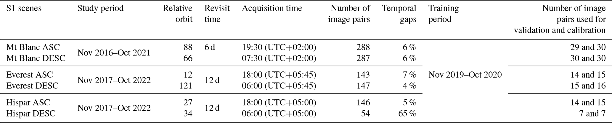
For each survey domain we derived the entire time series of Sentinel-1 images for the November 2017–October 2022 period for the two sites in HMA along two ascending and descending orbits and the November 2016–October 2021 period for the Mt Blanc region. We used one orbit for the ascending and descending tracks, 6 or 12 d apart, respectively, depending on the survey domain to guarantee that the incidence angles remained the same throughout the study periods. We used a different study period for the Mt Blanc region as Sentinel-1B experienced malfunction in December 2021, and the acquisition frequency dropped from 6 to 12 d over the European Alps (Table 1). This had little impact on the HMA sites, which had been monitored almost solely by Sentinel-1A, and only from the second half of 2017 at regular time intervals. Despite the systematic acquisition strategy, there were a few gaps (<10 %) in the time series of the Mt Blanc and Everest regions, which were more important in the descending acquisitions over Hispar (65 % gaps, with no images from October 2020 onwards, Table 1). For all three survey domains the ascending acquisitions were made late in the afternoon and the descending acquisitions early in the morning (Table 1).
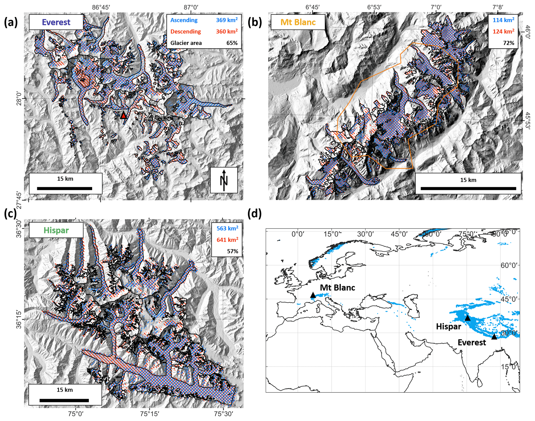
Figure 1The different survey domains on which the avalanche mapping was applied (a–c). The numbers in the upper-right corner indicate the total area of interest covered by the ascending and descending scenes, and the third number indicates the percentage of glacierized area covered by ascending or descending scenes. The Randolph Glacier Inventory (RGI) 6.0 outlines (RGI Consortium, 2017) are shown in black, the mapping extents for the ascending (descending) scenes are shown in blue (red). The red triangle in (a) indicates the location of the Pyramid precipitation gauge. The orange outline in (b) indicates the footprint of the Pléiades images. Background images are the AW3D30 30 m multidirectional hillshades. (d) Overview map of the three survey areas, with the RGI 6.0 glaciers indicated in blue.
Table 1Characteristics of the Sentinel-1 acquisitions in the ascending and descending orbits for each of the three survey domains.
In addition to the Sentinel-1 time series, we used four cloud-free Pléiades orthoimages acquired over the Mt Blanc massif with a spatial resolution of 0.5 m. Two images were taken during winter (8 December 2020 and 19 January 2021) and the other two during summer (8 July 2020 and 9 August 2020), and they were used to derive high-precision avalanche deposits to evaluate the outlines obtained with Sentinel-1. The winter and August Pléiades scenes were acquired on the same day as a Sentinel-1 acquisition, while the July scene was acquired 2 d before the nearest Sentinel-1 acquisition.
The characteristics of the avalanche deposits (size, elevation, slope) were derived using the global AW3D30 30 m DEM (Tadono et al., 2014). The avalanche time series obtained were also compared to the precipitation time series over the different study areas, as an indication of the amount of snow deposited at high elevations. For the Mt Blanc massif we used the rainfall and snowfall at 3000 m a.s.l. from the S2M reanalysis product (Vernay et al., 2022). For the Everest region we used precipitation measurements from the Pyramid precipitation gauge (Fig. 1a) with a Geonor sensor using a weighing device suitable for measuring liquid and solid precipitation (Khadka et al., 2022) located at 5035 m a.s.l. on the southern side of the survey domain. No station data were available for the Hispar region, so we used precipitation from the ERA5-Land reanalysis dataset (Muñoz Sabater, 2019).
3.1 Image pre-processing
All images were pre-processed in Google Earth Engine, using the S1 ground-range-detected (GRD) library (Gorelick et al., 2017). We filtered the images per orbit and kept only one ascending and one descending orbit per survey area to have observations at regular intervals (6 d for Mt Blanc, 12 d for Everest and Hispar). We conducted all the processing steps independently for the ascending and descending acquisitions. Images were mosaicked per day in case of overlapping images. We applied a 500 m high-pass filter to reduce the influence of large-scale snow wetness changes and averaged the VV and VH polarizations to reduce the speckle (Leinss et al., 2020). The backscatter values were then clamped to [−25, −6] dB, a range beyond which we do not expect to observe changes in the backscatter caused by changes in the snow surface roughness, and normalized to [0, 1] (Fig. 2). The images were then combined into RGB composites, with the backscatter of the D image (image taken on the day of interest) stored in the green channel and the D−i image (last image taken prior to the day of interest; i is equal to 6 or 12 d depending on the domain) stored in the red and blue channels. This enabled the identification of increases in the backscatter as green and decreases as purple (Fig. 3). We downloaded the first GRD images of each orbit from the Alaska Satellite Facility to produce a mask of shadow and layover using the ESA SNAP software. These masks were extended to all locations where the mean annual backscatter (brightness) was lower than 0.1, higher than 0.82, or outside the Randolph Glacier Inventory (RGI) 6.0 glacier extents (RGI Consortium, 2017) with a 200 m buffer (Fig. 1). As a result, 35 %, 28 %, and 43 % of the considered area were masked out for the Everest, Mt Blanc, and Hispar regions, resulting in a total area available for mapping of 492, 140, and 762 km2, respectively (Fig. 1).
3.2 Avalanche mapping
The mapping approach that we developed is adapted from the method by Karas et al. (2022) and as such uses the RGB images converted to hue, saturation, and value (HSV) space. This approach uses minimum saturation and value thresholds (TS and TV) to determine if the green patches in the image (which indicate an increase in the backscatter) should be classified as avalanche deposits. By targeting the saturation and brightness of these green patches, this approach is well suited to identify avalanche deposits in RGB images, with a true positive rate between 0.36 and 0.58 (Karas et al., 2022).
In this approach, which targeted the mapping of avalanche deposits over a multi-year period, we normalized the saturation and value by the mean values of the first images of the time series to improve the temporal consistency of the signal. We used a 35° slope threshold above which the increases in backscatter were not considered to be avalanche deposits and removed all detections smaller than 40 pixels (4000 m2; Leinss et al., 2020; Eckerstorfer et al., 2019). Furthermore, in addition to the two thresholds on saturation (TS) and value (TV) proposed by Karas et al. (2022), we added extra constraints to reduce the effect of changes in snow wetness, which would otherwise lead to a large number of false positive detections. First, once the bright green patches had been detected, we allowed them to expand within a vicinity of 7 pixels (70 m) to capture less bright parts of the avalanche deposit according to another threshold value TO, identical for both the saturation and value (Fig. 2, second filtering step). Second, we directly differentiated the image at D with low-pass-filtered images at D and D−i (Sm D and Sm D−i). The low-pass filter consisted of a 45-pixel-wide (450 m) Gaussian filter. We selected this kernel size to be able to smooth even the largest avalanche deposits. We kept only pixels for which at least one of the differences was above set thresholds (TD1, TD2, and TD3, third filtering step, Fig. 2). The idea of this additional step was that an avalanche event results in a spatial discontinuity in the backscatter, if not with the image before, then at least in the current image.
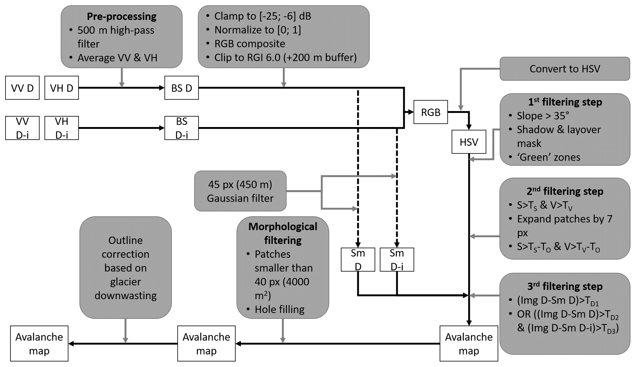
Figure 2Processing steps (grey) applied to the Sentinel-1 GRD data (white) to obtain avalanche maps. The polarizations VV and VH at D (image taken on the day of interest) and D−i (last image taken prior to the day of interest; i is equal to 6 or 12 d depending on the domain) are averaged to get backscatter (BS) images, which are then combined into an RGB and then an HSV image. These HSV images are then filtered following three filtering steps using six different thresholds (TS, TV, TO, TD1, TD2, and TD3) before the final morphological filtering step and correction for glacier elevation change. Sm indicates the smoothed images after application of the 45-pixel low-pass filter.
3.3 Parameter calibration
We manually derived the avalanche deposit outlines of all images between November 2019 and October 2020 at all sites, based on the pre-processed RGB images. The main advantage of the manual mapping is that it gives the possibility to account for the shape of the events to discriminate avalanche deposits from changes in snow wetness, for example (Vickers et al., 2016; Eckerstorfer et al., 2016; Hafner et al., 2021). A single operator performed the manual detection, and to account for biases in the delineations, we compared on a pixel-by-pixel basis these outlines with those of four other operators for four scenes (two ascending and two descending) covering the Mt Blanc region and four scenes covering the Everest region (Kneib et al., 2021; Table S1 in the Supplement, Figs. S2–S3).
The manual outlines were used to calibrate and validate the six free parameters (TS, TV, TO, TD1, TD2, and TD3) used for the mapping (Fig. 2). We used the F1 score, also known as the Dice coefficient, as a metric to quantify the goodness of fit of the automated delineation on a pixel-by-pixel basis (Dice, 1945; Sørensen, 1948):
where TP is the number of pixels classified as true positives, FP as false positives, and FN as false negatives (Fig. 3). This metric is therefore well suited when the mapping targets represent a small percentage of the total area of the scene, and a calibration based on this metric will result in finding the parameters that lead to maximizing the number of TP while also balancing the number of FP and FN (Kneib et al., 2020). For a perfect classification, the F1 score is equal to 1.
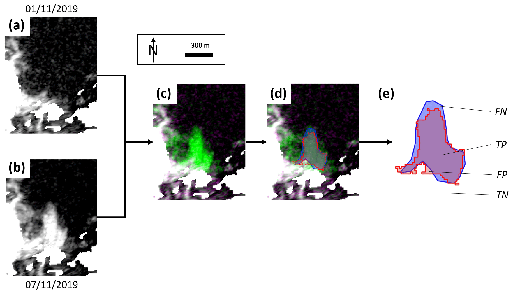
Figure 3Example of the different processing steps from two pre-processed Sentinel-1 images taken at a 6 d interval (a, b), combined into one RGB image for change detection (c). The different bands range between −25 and −6 dB. This image is then used for the manual (blue outlines) and automated (red outlines) mapping of the avalanche deposits that appear in green (d). These outlines are then compared based on the confusion matrix, used to compute the F1 score, with TN corresponding to the true negative pixels, TP to the true positive pixels, FP to the false positive pixels, and FN to the false negative pixels (e).
We used every second image pair for the calibration, and the remaining half was used for validation (∼28 pairs for Mt Blanc and ∼14 for the Hispar and Everest regions for ascending and descending scenes). We split the time series into two time periods, November–April and May–October, to account for lower backscatter values across large portions of the glaciers during the melt season, which we considered to be bounded by the May–October period for all survey domains (Karbou et al., 2021; Scher et al., 2021). Thus, the calibration and validation were done independently for each ascending and descending orbit of each survey domain and for each time period. We started from an initial guess of all parameter values (TS, TV, TO, TD1, TD2, and TD3) based on trial and error and then randomly sampled the parameter space within reasonable bounds (Fig. 2), using the following ranges of value ([min, max]) obtained from trial-and-error tests: [0.20, 0.65], [0.20, 0.65], [0.01, 0.16], [0.05, 0.11], [0.01, 0.09], and [0.31, 0.43]. For each survey area and each orbit, we chose the set of parameters that maximized the F1 score. This parameter selection was then evaluated against the validation set and used to automatically map avalanche deposits across the entire Sentinel-1 time series.
Of all six parameters used for the calibration, the saturation threshold TS was the only one with a defined value maximizing the F1 score, between 0.3 and 0.5 (Fig. S4), and therefore also the most sensitive. The other parameters did not have a clear maximum defined, and several combinations of these parameters could lead to similarly high F1 scores (Figs. S5–S9).
3.4 Comparison with optical images
We compared on a pixel-by-pixel basis the Sentinel-1 outlines that occurred over given periods in the summer and in the winter with manually derived outlines of avalanche deposits from high-resolution (0.5 m) Pléiades orthoimages over parts of the Mt Blanc survey area, acquired on 8 December 2020, 19 January 2021, 8 July 2020, and 9 August 2020. We also compared the aggregation of 1 year (November 2019–9 August 2020) of Sentinel-1 manual outlines from ascending and descending orbits with all the avalanche deposits identified in a Pléiades image taken at the end of the summer season (9 August 2020), with the assumption that these end-of-summer deposits result from the union of all individual deposits throughout the year. This comparison was made for all deposits above 2700 m a.s.l., which was the altitude of the snowline, derived from the Pléiades orthoimage. We also restricted the comparison to locations with slopes lower than 35° and within the ascending or descending mapping extents (Fig. 1). We attempted to do the same over the Everest survey domain using 5 m resolution Venus multi-spectral images (Raynaud et al., 2020) but found that the spatial resolution was not high enough to outline the deposits with a high enough confidence. For the Hispar region, there were also no such high-resolution (<5 m) optical images available for the study period.
3.5 Application to entire Sentinel-1 time series
After calibration and validation of the mapping approach, we applied it to a 5-year time series of Sentinel-1 images over the three survey domains (Table 1), using 6 d intervals for the Mt Blanc region and 12 d intervals for the Everest and Hispar regions. We required highly accurate maps of avalanche deposits for the analysis of their spatio-temporal characteristics. False positive (including from crevassed areas, changes related to snow wetness, vegetated areas, frozen supraglacial lakes) and false negative detections were corrected manually to obtain a dataset comparable to the November 2019–October 2020 calibration and validation dataset. The Google Earth Engine Sentinel-1 images are map projected using the Shuttle Radar Topography Mission DEM, so we had to account for glacier elevation change by shifting the outlines based on the local elevation change rates from Hugonnet et al. (2021) and the Sentinel-1 look and heading angles for each orbit (Fig. S10). While these shifts were negligible in the accumulation area of most glaciers, they reached values of 5 m yr−1 in the lower ablation zone of the glaciers in the Mt Blanc region, which had the highest surface lowering rates. The final outlines were aggregated into avalanche “activity” maps indicating the avalanche frequency for the different avalanche deposits.
3.6 Characterization of avalanche activity
The union of all avalanche pixels over time indicates individual deposits affected by more or less avalanche activity. We estimated the influence of avalanches on a given glacier, independently for ascending and descending orbits, with two metrics: area affected by avalanches and avalanche activity. The area affected by avalanches is estimated by taking the union of all individual avalanche deposits and is expressed relative to glacier area. The avalanche activity is calculated for each pixel as the number of avalanches affecting this pixel over a given time period. It is then calculated on a per-deposit basis by taking the maximum activity and on a per-glacier or per-elevation band basis by taking the area of the glacier affected by avalanches divided by glacier area or area of elevation band, respectively. We also defined a catchment for each glacier by taking all its upstream area following the D-infinity method (Schwanghart and Scherler, 2014). We could then calculate for each glacier the ratio (R) of the area of the catchment with slopes steeper than 30°, which stands as a proxy for the avalanche contribution area and the glacier area (Hughes, 2008; Laha et al., 2017).
Here, we first compare our manually derived outlines with high-resolution Pléiades images and evaluate the performance and transferability of the automated mapping approach (Sect. 4.1). We then use the manually updated set of outlines to obtain the characteristics of avalanche deposits (Sect. 4.2) and their spatio-temporal variability (Sect. 4.3) for all three survey domains.
4.1 Sentinel-1 avalanche mapping
4.1.1 Comparison of Sentinel-1 and Pléiades manual detections
The qualitative comparison of the manually derived Sentinel-1 deposits with the Pléiades deposits detected over time periods of ∼1 month in the winter and summer seasons gives more insights into the potential of Sentinel-1 images to identify particular deposits (Fig. 4). It indicates locations of very good agreement, usually for large deposits with a lot of surface texture (Fig. 4c). But there are also false positive detections, for example caused by the opening of crevasses (Fig. 4b), and false negatives (Fig. 4a), which could reach large sizes (up to 60 000 m2, Fig. 4d). The comparison of the aggregation of 1 year of Sentinel-1 manual outlines with all the deposits identifiable in the end-of-summer Pléiades scene above 2700 m a.s.l. results in an F1-score value of 0.47, with a majority of false negatives (Fig. S11). A large amount of deposits identified in Pléiades but not Sentinel-1 is smaller than the Sentinel-1 detectability threshold of 4000 m2. Nevertheless, excluding them does not change the comparison (F1-score value of 0.49) between the Pléiades and aggregated Sentinel-1 deposits.
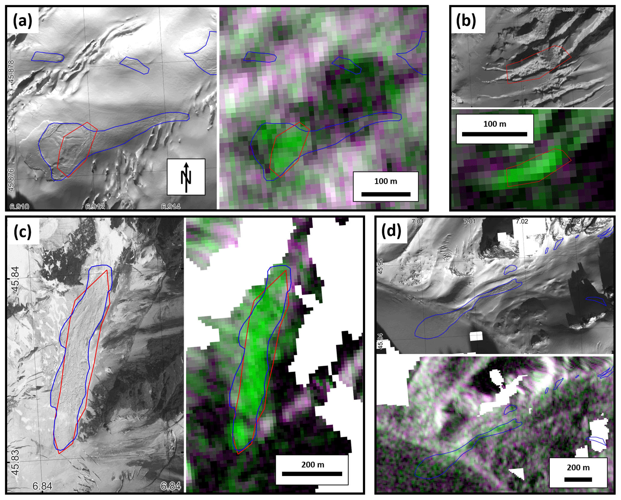
Figure 4Examples of manual avalanche detections in the Sentinel-1 (red) and Pléiades (blue) images (© CNES, distribution AIRBUS DS): (a, d) Dry-snow avalanches are clearly identifiable in the Pléiades images, but only the deposits with high surface roughness are visible in the Sentinel-1 RGB images; (b) false positive detection of an opening crevasse in Sentinel-1; and (c) large avalanche deposit clearly visible in both Pléiades and Sentinel-1 imagery.
The comparison of the manual outlines from four independent operators provides some insights into potential biases of the manual delineation. The F1 scores of the three external operators relative to the main operator that derived the entire manual dataset for all three sites range between 0.54 and 0.66 (Table S1, Figs. S2–S3). We also directly compared the manual outlines from this operator with the consensus outlines from the other three operators, which were the outlines for which at least two operators agreed (Kneib et al., 2021). The outlines used for the calibration and validation of the automated mapping approach lead to less avalanche detections ( % of events detected and % of deposit areas) than the consensus outlines and can therefore be considered to be a lower bound for the manual detection of avalanches in the Sentinel-1 RGB pairs.
4.1.2 Evaluation of the automated mapping approach
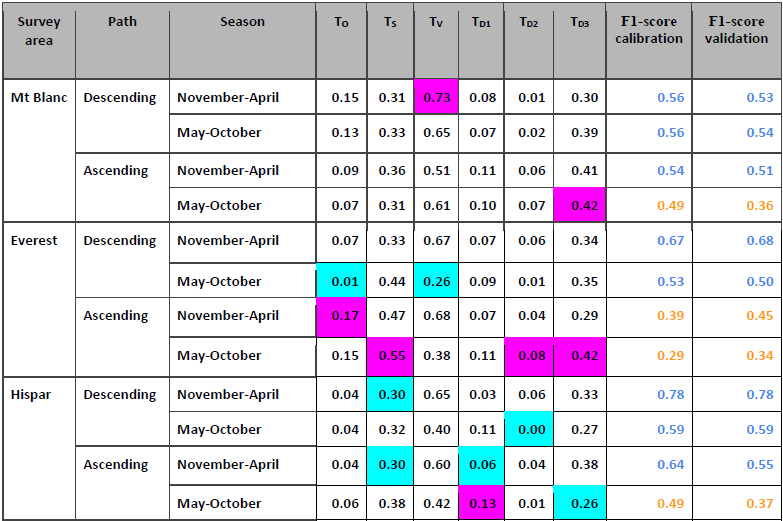
We obtained F1 scores ranging between 0.29 and 0.78 when calibrating the mapping parameters against the manually derived outlines from Sentinel-1 (Table 2). The F1 scores are similar for both calibration and validation sets, which indicates the good transferability of the parameters between scenes taken during the same season and with the same orbit. F1 scores are generally lower for the ascending orbits (average F1 score of 0.47) compared to the descending ones (0.62) and for the warm season (0.49) compared to the cold season (0.60). Except for the Everest ascending scenes, the F1 scores obtained for the calibration were always higher than 0.49.
Table 2Results of the calibration and validation of Sentinel-1 avalanche outlines for the November 2019–October 2020 period for each of the three survey areas. The values of the calibrated parameters are indicated along with the F1 scores obtained for the calibration and validation sets. For each parameter the minimum value obtained is indicated in cyan and the maximum in magenta. F1 scores are written in blue when they are higher than 0.5 and in orange when lower.
Local increases in the Sentinel-1 backscatter that are discarded in the manual delineation but that can be detected as false positives in the automated approach can in some cases be linked to widespread snow backscatter increases, likely due to wetness changes, especially during the May–October season (Fig. S12a), or calving into proglacial lakes (Fig. S12b). Conversely, the automated approach could miss events which had backscatter values below the imposed thresholds but had the obvious shape of an avalanche (Fig. S12c). Such false positive or false negative detections were manually removed or added based on considerations of shape, size, and location, and this manual filtering was applied to all time series of all survey domains for the results presented in Sects. 4.2 and 4.3. Over the entire automatically derived dataset we removed 36 % of the mapped deposits and added 41 % of what we considered to be false negatives (Fig. S13). Furthermore, we also observed that deposits with a high avalanche activity remained with a high backscatter value for time periods of several months during which there was not enough time, surface melt, or precipitation for the surface roughness of the deposits to change significantly between two Sentinel-1 acquisitions. The only way that avalanches can be detected on such deposits is when they are large enough to have their runout zone go beyond the previous avalanche deposits (Figs. S12d, S14). Therefore, for many deposits across the three survey domains, the frequency and size of avalanche events are likely to be underestimated.
We compared the total size and number of manually and automatically derived avalanche events for the Sentinel-1 validation image sets over the November 2019–October 2020 period (Figs. 5, S15–S17). There is a relatively good correspondence between the two categories for the Mt Blanc region and the Everest and Hispar regions during the cold and warm seasons, with Pearson's correlation coefficients (Pearson, 1895) higher than 0.85 for the total size and 0.71 for the number of detected deposits. The automated mapping generally underestimates the number and sizes of the avalanche deposits, especially in the May–October season, which is due to conservative thresholds to reduce the false positive detections of snow wetness changes (Figs. 5, S15–S17). But it provides a good estimate of temporal variability in avalanche activity, as shown by the high correlation scores.
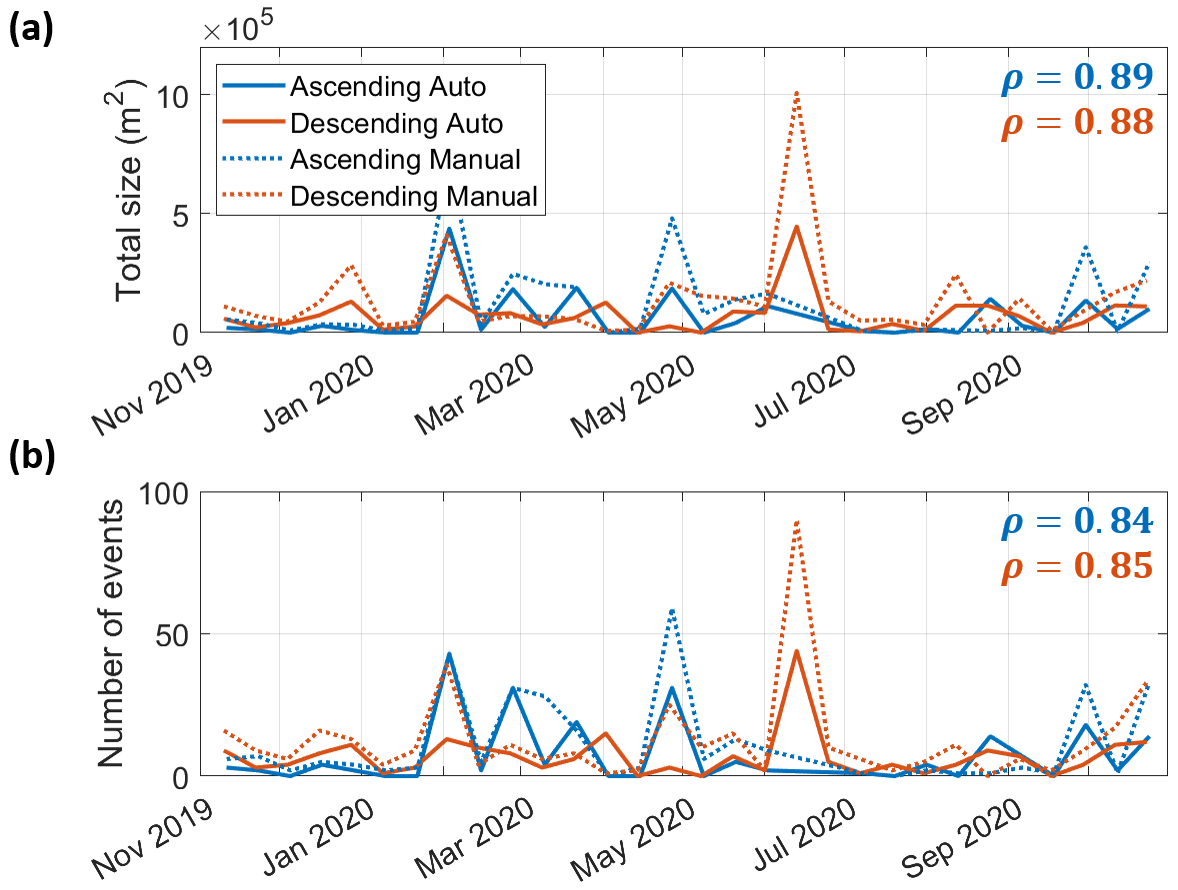
Figure 5Total size and number of manually and automatically detected avalanche events as a function of time for the November 2019–October 2020 period for the validation datasets of Mt Blanc. Pearson's correlation coefficients characterizing the correlation between the validation set and the outlines from the automated mapping approach are indicated in blue (ascending) and red (descending).
4.1.3 Transferability of the automated mapping parameters
To test the transferability of the calibrations obtained for the different orbits and periods of the different survey domains, we applied these parameterizations to the other survey domains, including the Mt Blanc scenes with a 12 d interval (Table 3), without any manual edits. Most parameterizations are well transferable to the Hispar and Everest November–April descending scenes and the Hispar May–October descending scenes, with F1 scores above 0.5 in 78 % of the cases (0.6 in 83 % of the cases for the Hispar November–April scenes). The ascending scenes present in general lower F1 scores (lower than 0.5 in 92 % of the cases), particularly the May–October scenes of Everest, for which the F1 score never exceeds 0.32. With an average F1 score of 0.46, the Everest descending November–April parameter set is the most transferable but still performs poorly (F1 score <0.4) for some of the ascending and/or May–October scenes (Table 3).
Table 3F1 score obtained when applying different sets of parameters to sets of images for which they were not calibrated, without any manual edits. The parameters in the last column correspond to the median parameters calibrated over Mt Blanc (6 d intervals), Everest, and Hispar. The diagonal values correspond to the calibrated parameter sets for the given study area, orbit, and period. N–A and M–O stand for the November–April and May–October periods, respectively.
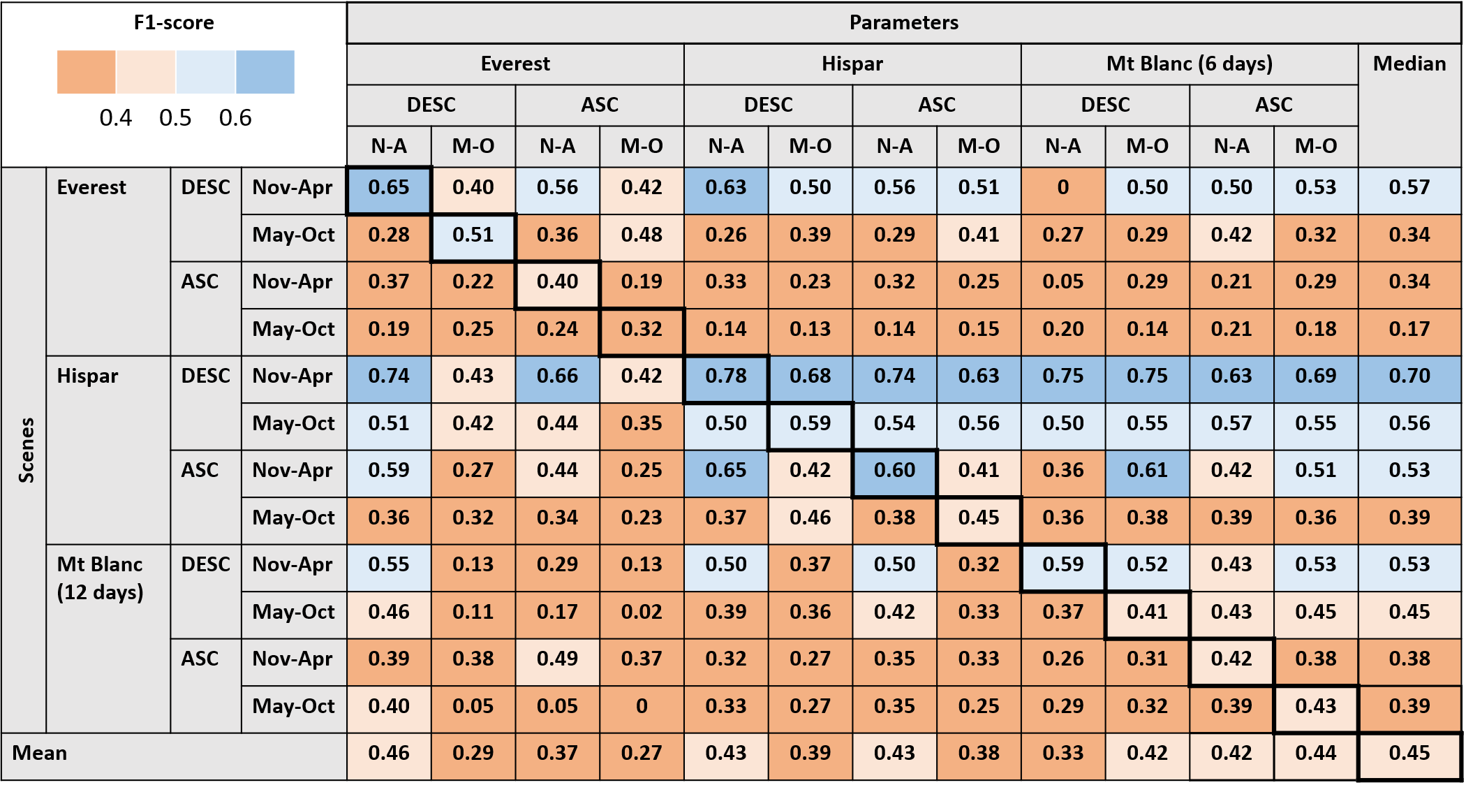
The F1 scores obtained for Mt Blanc with a 12 d interval are maximized by the Mt Blanc 6 d parameters but with generally lower F1 scores than the ones obtained for the Mt Blanc scenes with a 6 d interval (Table 2). The application of the different parameter sets to the Mt Blanc 12 d scenes results in more false positive detections than false negatives (Table S2).
4.2 Characteristics of avalanche deposits
After manually editing the automated outlines, we detect 1801 (2761) avalanche events in the Mt Blanc region, 1192 (2808) in the Everest region, and 4323 (3417) in the Hispar region with the ascending (descending) scenes, corresponding to , , and avalanches m−2 yr−1 in the ascending and , , and avalanches m−2 yr−1 in the descending orbits in the three above-mentioned regions, respectively.
Due to the time frequency of images, there appear to be more avalanches detected over Mt Blanc than over the two HMA domains (Fig. 6a). The size distribution of the avalanches follows a similar distribution for the different regions, at least beyond the 4000 m2 detectability thresholds (Fig. 6b). These distributions followed an exponential decrease, with slopes between m−2 for Hispar and m−2 for Mt Blanc, with a coefficient of determination (R2) between 0.44 and 0.89 (Table S3). Some of the largest events (up to 1.0×10⁶ m2) are found in the Hispar region, which is also the region with the highest number of detected avalanches relative to the area and number of image pairs. The distribution of avalanches is closely related to the hypsometry of the surveyed areas (which correspond to the buffered glacierized areas without the shadow and layover masks), although for all three survey domains, and for the Mt Blanc region in particular, the peak in avalanche activity is generally slightly lower than the peak in hypsometry (Fig. 6c). The elevation range over which avalanches are actively detected is narrower than the catchments' hypsometry for Everest and Hispar, where avalanches proportionally affect the upper elevations less, which are also the steepest (Fig. S1b), and where there are extensive and relatively flat glacier tongues with no visible avalanche activity. This is not the case for the Mt Blanc massif where avalanches are the most frequent at lower elevations, relative to the hypsometry.
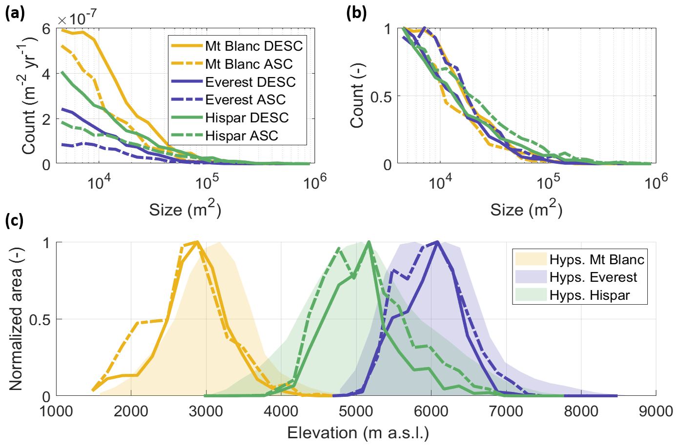
Figure 6Size distribution of avalanche events at the three different sites, with (a) and without (b) normalization. (c) Normalized area of all avalanche events expressed as a function of the surveyed area segmented into 200 m elevation bins. The legend in panel (a) applies to all three panels.
Avalanche deposits have a maximum activity of 3.8 events per year for the Mt Blanc massif and up to 4.6 events per year for the Hispar and Everest regions, where Sentinel-1 image pairs are acquired at a 12 d interval (Fig. 7a). These maxima are likely an underestimation of the actual deposit activity given that deposits with frequent avalanche activity remain with high surface roughness and therefore high backscatter values for long periods of time, preventing the detection of further avalanches (Figs. S12c–d, S14). Despite these limitations, distributed deposit activity maps are indicators of where the most active avalanche deposits are located, which is generally at the base of steep headwalls and in some cases below large hanging glaciers (Fig. 7b–e).
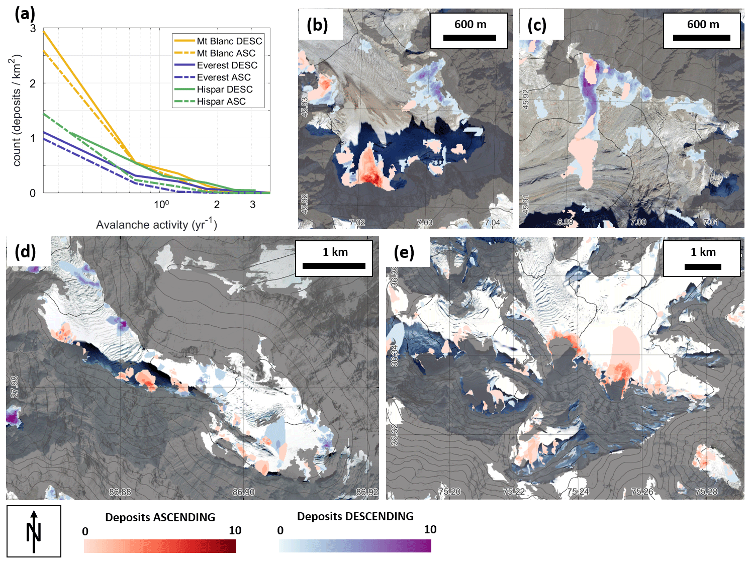
Figure 7(a) Avalanche activity for all avalanche deposits. (b–e) Examples of avalanche activity maps (number of avalanches over the 5-year study period) at various locations across the three survey domains, on the Argentière Glacier (b) and the Talèfre Glacier (c) in the Mt Blanc region, on the Khumbu Glacier (d) in the Everest region, and on the Mulungutti Glacier (e) in the Hispar region. Deposits detected in the ascending images are shown on top of the deposits detected in the descending images. The contour lines are from the AW3D30 DEM and are taken every 200 m. The background images are from © Google Earth. The grey-shaded areas correspond to the intersection of ascending and descending masks.
We compared the avalanche activity and proportion of avalanche deposits on the different glaciers of the three survey domains with the proportion of slopes steeper than 30° in the glaciers' catchments (R index, Hughes, 2008; Laha et al., 2017). We found that for a given proportion of steep slopes, the maximum avalanche activity and proportion of avalanche deposits per glacier are generally around 1 order of magnitude smaller than this R index (Figs. S18–S19). It is also noteworthy that a number of (generally smaller) glaciers have an avalanche activity and proportion of avalanche deposits smaller than this maximum value, indicating that while a high R-index value is a necessary condition for high avalanche activity, it is not sufficient.
4.3 Spatio-temporal evolution of avalanches
The avalanche activity varies seasonally and with elevation. There are pronounced seasonal differences (Figs. 8–10, S21–S23, Table S4) enhanced by the interannual variability of deposit activity (Fig. S20). Interestingly, only a minority of deposits are active every year, which indicates that the detected yearly avalanche activity at a given location is not very regular (Fig. S20).
At all three sites, the spatio-temporal patterns in the number and size of detected avalanche events are similar from year to year (Figs. 8–10, S21–S23). There are avalanches all year round over the Mt Blanc massif but with a higher activity between January and July (Figs. 8, S24–S28). Between January and April there are well-individualized peaks in avalanche activity, which correspond to peaks in solid precipitation and are well captured by the avalanche forecast (Figs. S26–S28). From mid-April to July, despite the lower amount of precipitation (Table S5), there are longer periods of avalanche activity with a similar number and size of events as in the colder January–March months but which are not captured by the avalanche forecast (Figs. S26–S28, Table S4). From mid-November to mid-April, avalanches are mostly identified at elevations lower than 3500 m a.s.l. and as low as 1500 m a.s.l., which is the lowest elevation reached by glaciers in this survey domain (Fig. S1). This lower limit of avalanche detections rises from 1500 to 2700 m a.s.l. between April and July, and from mid-June the avalanche activity reduces, and all events take place between 2700 and 4300 m a.s.l. The avalanche activity increases again from December onwards, and the elevation of detected avalanches lowers again to 1500 m a.s.l. by January. Peaks in avalanche activity generally correspond to peaks in precipitation, including during the warmer months of April–July (Figs. S24–S28).
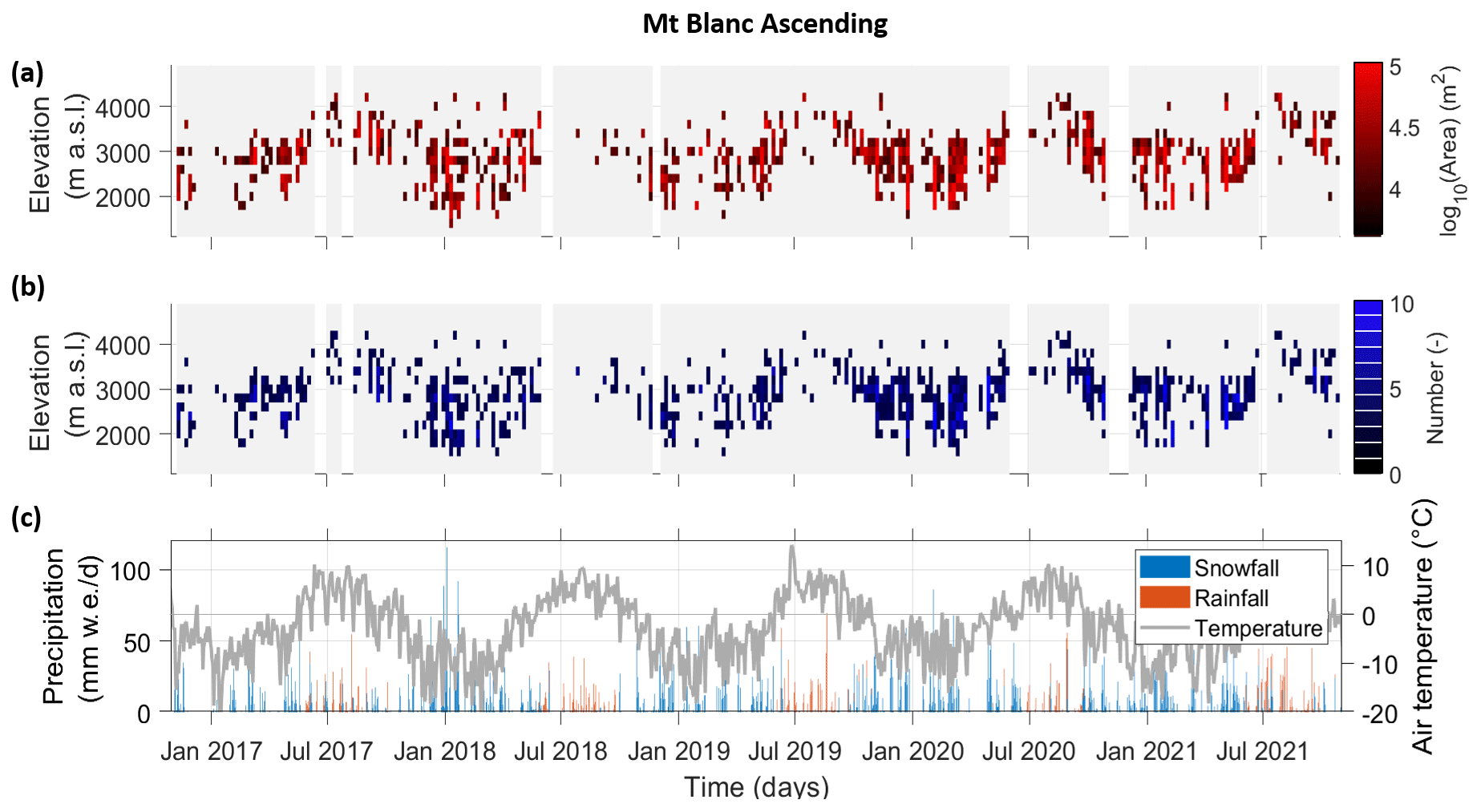
Figure 8The 5-year (November 2016–October 2021) avalanche time series over the Mt Blanc massif in the ascending orbits. (a) Total area and (b) number of avalanches as a function of time and elevation for each Sentinel-1 pair. Frequency of acquisitions is 6 d. The white rectangles indicate data gaps. (c) Total precipitation and mean daily air temperature at 3000 m a.s.l. over the Mt Blanc massif according to the S2M reanalysis product (Vernay et al., 2022).
A seasonality is also apparent for the Everest region, with the highest avalanche activity occurring in the monsoon months, between 21 June and 21 September (45 %–53 % of the annual avalanche activity, Table S4), with a ∼1-month lag relative to the start of the monsoonal precipitation events (Figs. 9, S22, Tables S4–S5), with some high pre-monsoon precipitation events such as at the end of May 2021 seemingly not affecting the avalanche activity. This is also when avalanches are detected at higher elevations, between 5300 and 7100 m a.s.l. During the periods from October to April avalanches range between 5100 and 6300 m a.s.l. and are much less frequent, with periods with no detected avalanches at all.
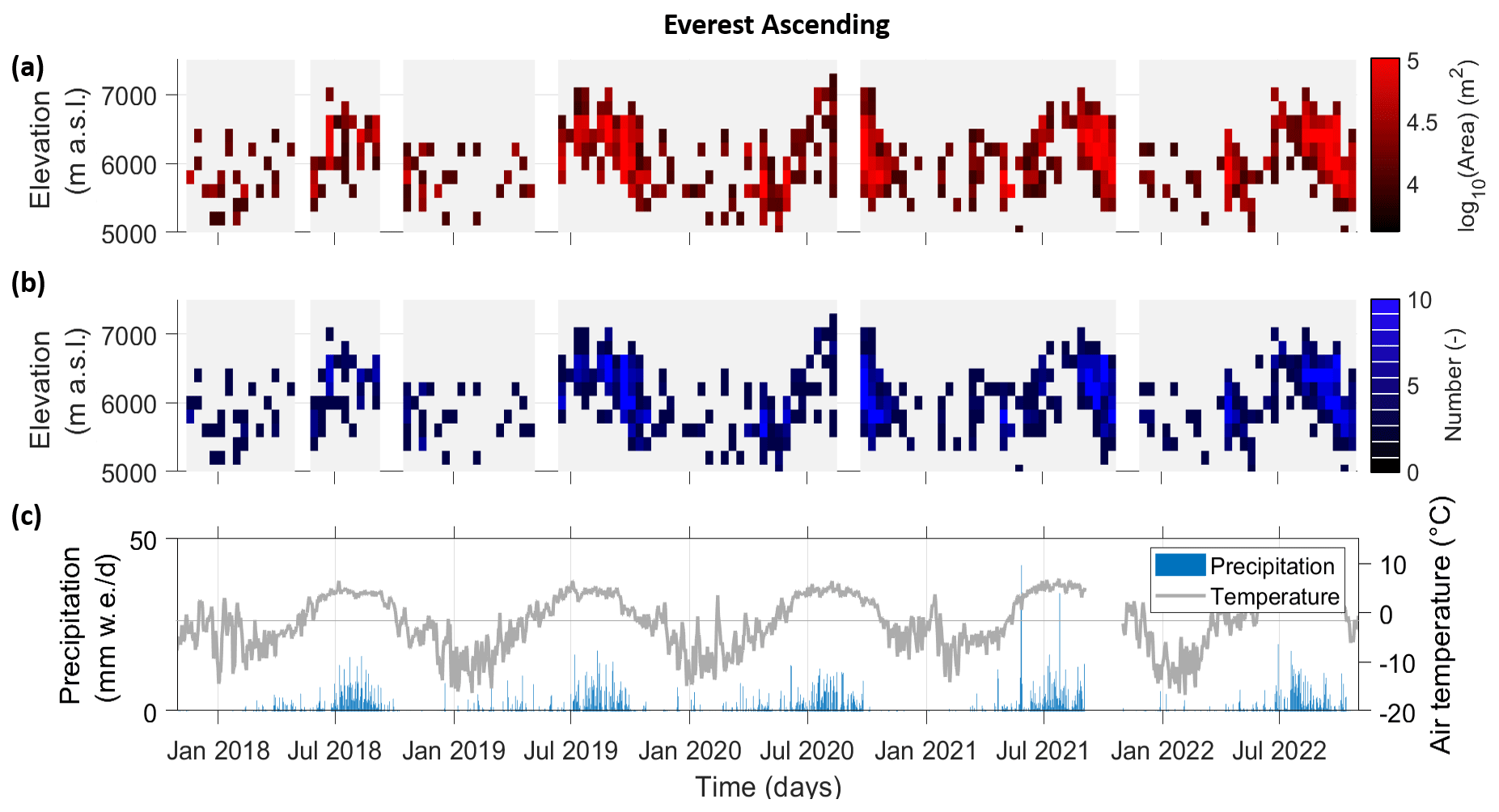
Figure 9The 5-year (November 2017–October 2022) avalanche time series over the Everest region in the ascending orbits. (a) Total area and (b) number of avalanches as a function of time and elevation for each Sentinel-1 pair. Frequency of acquisitions is 12 d. The white rectangles indicate data gaps. (c) Daily precipitation and mean air temperature recorded at the Pyramid precipitation gauge (5035 m a.s.l.).
There is also a seasonal signal visible for the Hispar domain, mostly linked to temperature and snow conditions as precipitation occurs all year round without a clear seasonality (Fig. 10, Table S5). The avalanche activity is the highest between May and October, which is also when air temperatures are higher, and avalanches are detected at higher elevations, between 4500 and 6700 m a.s.l. This lower-elevation bound does not vary much during the year; however, the upper-elevation bound lowers down to 5300 m a.s.l. during the cold period between October and May, even if it is less defined than for the other two survey domains.
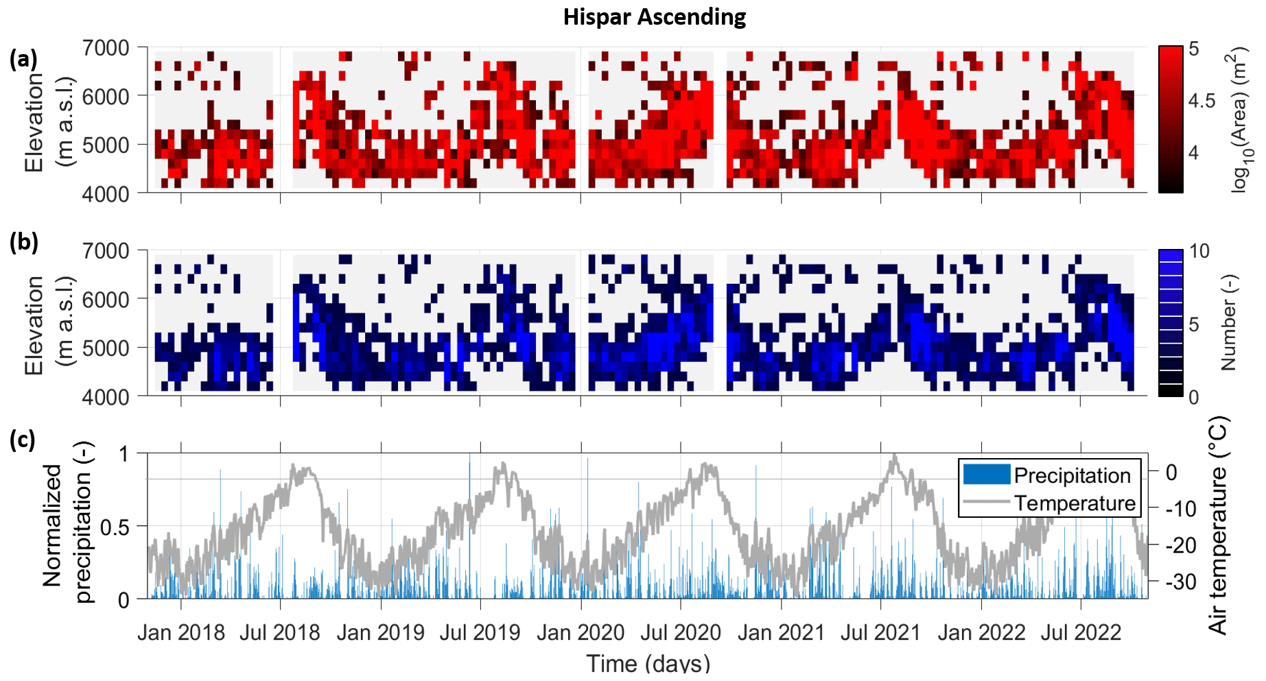
Figure 10The 5-year (November 2017–October 2022) avalanche time series over the Hispar region in the ascending orbits. (a) Total area and (b) number of avalanches as a function of time and elevation for each Sentinel-1 pair. Frequency of acquisitions is 12 d. The white rectangles indicate data gaps. (c) Daily precipitation and mean air temperature over the region are from the ERA5-Land reanalysis product (Muñoz Sabater, 2019). Daily precipitation values were normalized due to potential biases (Khadka et al., 2022).
5.1 Suitability of Sentinel-1 for detecting avalanches in remote glacierized regions
We have applied a semi-automated approach to obtain a long-term (5 years) time series of avalanche deposits in remote glacierized areas of the European Alps and High Mountain Asia, locations where few data on such events existed.
We used Sentinel-1 images to detect avalanche events, which enabled us to obtain a massif-wide distributed dataset, at least for the zones unaffected by shadow and layover (57 %–72 % of our survey domains characterized by steep topographies). This dataset is therefore less spatially biased than ground-based inventories in populated valleys (Eckert et al., 2010; Schweizer et al., 2020). Our comparison of the Sentinel-1 with the Pléiades avalanche deposit outlines indicates that avalanches detected with Sentinel-1 are of relatively large size (>4000 m2 deposits) with high surface roughness, which limits the detectability to avalanches with high enough snow temperatures to form granular deposits (Steinkogler et al., 2015), avalanches that are formed from cohesive wind slabs (Fig. 4a), or avalanches that entrain rock or ice debris (for instance from serac falls; Fig. 4c). Therefore, cold, low-density snow progressively redistributed down steep rock faces or snow gullies (Sommer et al., 2015) is likely to be missed by this method, which likely also explains the upper-elevation limits to avalanche detections, especially during the cold season (Figs. 8–10). Similarly, the detection of the avalanche events requires the previous deposits to have regained lower backscatter values for the signal to be visible, meaning that the surface of the deposit needs to have been smoothed by additional precipitation or melt for the next events to be visible at this location. We have observed this smoothing to require several weeks or even months before avalanches can be detected at the location of old deposits; meanwhile, new avalanche events continue to occur, therefore making detection difficult (Figs. S12d, S14). In other cases, high wind speeds or new precipitation are likely to mask the deposits in the time interval of 6 to 12 d. The avalanche activity that is detected is therefore a lower-bound value of the actual avalanche activity, and the aggregation of all Sentinel-1 deposits is still an underestimation of all the glacierized areas affected by gravitational snow redistribution (Fig. S11). It is also noteworthy that this mapping approach with Sentinel-1 will likely not differentiate large rockfalls on glaciers from snow avalanches, which could explain some of the activity in the summer and autumn in the Mt Blanc massif. Nevertheless, this semi-automated approach is promising for exploring the temporal and spatial variability of avalanches in remote areas, especially in glacierized regions of HMA, where close to no data exist on the occurrence of such events (Ballesteros-Cánovas et al., 2018; Caiserman et al., 2022; Acharya et al., 2023; Singh et al., 2022).
The performance metrics obtained from our automated mapping approach compared to the manual detections in the Sentinel-1 outlines have a wide range of values (F1 score between 0.29 and 0.78) depending on the season and acquisition time. For most scenes, the F1 score was similar to the scores obtained by manual outlines from independent operators (Table S1, Hafner et al., 2023). These results are similar to those of other studies following similar threshold-based approaches (Leinss et al., 2020; Eckerstorfer et al., 2019; Karas et al., 2022; Wesselink et al., 2017). The performance of such approaches is generally very good in dry-snow conditions, with high precision (>0.7) and low false positive rates (<0.4), which correspond to F1 scores above 0.6–0.7 (Leinss et al., 2020; Eckerstorfer et al., 2019). Therefore, while dry-snow conditions lead to detectability limitations in Sentinel-1 images (Fig. 4), when avalanches are manually detected in Sentinel-1 scenes in dry-snow conditions, they are usually also well mapped by the automated approach, as indicated by the high F1 scores (Eckerstorfer et al., 2022). The few studies that targeted extensive periods rather than a specific event also encountered the most difficulties for periods with wet-snow conditions, leading to extensive false positive detections which had to be removed manually in situations of dry- to wet-snow transitions (Eckerstorfer et al., 2019). Such false positive detections can be discarded manually based on size and texture considerations, which indicates that deep-learning approaches based on convolutional neural networks, for example, offer a promising way to improve these classifications (Tompkin and Leinss, 2021; Waldeland et al., 2018; Yang et al., 2020; Bianchi et al., 2021; Kapper et al., 2023; Liu et al., 2021; Lê et al., 2023). Such machine learning approaches trained with large enough datasets (Hafner et al., 2021) would likely also improve the transferability of the mapping to other sites with different topo-climatic conditions and frequency of acquisitions. Indeed, scenes unaffected by snow wetness changes (descending/morning acquisitions during the cold season) are well mapped regardless of the parameter set (Table 3). Ascending scenes, acquired in the afternoon, are more likely to be affected by snow wetness changes than descending scenes, acquired in the morning, which explains the lower F1 scores for these scenes.
For future implementation of SAR detection of avalanches, we therefore recommend prioritizing the use of morning-to-morning scenes. Although scenes acquired in the afternoon may help fill spatial and temporal gaps and could be used as a confirmation for some detections, it is important to note that they will require additional work to separate actual avalanche events from false positive detections caused by snow wetness changes. This is a difficult task, leading to higher uncertainties in the mapping, and will likely not considerably change the long-term spatio-temporal patterns in avalanche activity (Figs. 8–10). At this stage, automated outlines need to be carefully checked manually even during the cold season and for the morning scenes, with up to 36 % of false positive detections and 41 % of false negative detections for our survey domains (Fig. S13). Our semi-automated mapping therefore still requires manual edits, although we consider that applying the automated mapping approach and then updating the outlines by hand have reduced the mapping time by at least half relative to a fully manual mapping, more if only morning scenes were to be considered. Similarly, the parameters used for the automated mapping are likely not directly transferable to other locations. However, using the median of all our parameter sets (Table 2) is likely a good first guess to apply our mapping approach to other survey areas (Table 3), either for the calibration of new parameters or to obtain a first reasonable avalanche map which can then easily be updated manually. Future method developments could also benefit from separating the VV and VH polarizations, particularly for regions of the SAR images with low incidence angles (Tompkin and Leinss, 2021). While in our case we obtained better results by averaging the two polarizations (Table S7), other machine-learning-based approaches would likely benefit from the additional information provided by the two polarizations (Liu et al., 2022). In the end, this study resulted in a manually checked dataset of 16 302 avalanche deposits, which will be highly beneficial for the training of future mapping approaches.
5.2 Characteristics of on-glacier avalanches
The size distribution of avalanches with Sentinel-1 RGB pairs reaches a maximum around 4000 m2 (avalanches smaller than 4000 m2 have been filtered and are therefore not considered in this study). Beyond this 4000 m2 value the frequency of avalanches decreases with size, following a similar exponential decrease for all survey areas (Fig. 6, Table S3). Similar observations have been made for snow avalanches in the European Alps and North America based on field inventories (Faillettaz et al., 2004; Birkeland, 2002; Schweizer et al., 2020). The lower number of small avalanches in these inventories is generally interpreted as an observation bias, with small events being difficult to detect visually and not consistently inventoried (Schweizer et al., 2020), unless automatically recorded by seismic sensors (Reuter et al., 2022). This is also the case for detections of avalanches (or any other features) using remote sensing products, which are constrained in this case by the spatial resolution of the images (Hafner et al., 2021; Miles et al., 2017; Kneib et al., 2020). The 4000 m2 threshold was therefore interpreted as a size detectability threshold below which avalanches are likely to be missed. This value is consistent with other studies that have used Sentinel-1 images for the detection of avalanches (Eckerstorfer et al., 2019).
During the periods with the highest avalanche activity in the three survey domains we detected between 2 (Everest) and 8 (Mt Blanc) avalanches per day per 100 km2, which is relatively low compared to the value of 10–20 avalanches per day per 100 km2 suggested by Schweizer et al. (2020) for days with a high avalanche level (4) in the Davos region of Switzerland. This difference is likely due to the detectability threshold and the fact that recurring avalanches are likely to be missed if the surface roughness does not change between two events (Figs. S12c–d, S14). More avalanches are detected in the Mt Blanc massif, which is likely at least partly due to the higher temporal frequency of Sentinel-1 acquisitions over this range. Indeed, manual mapping of avalanches with images with a 12 d interval results in 4 % to 62 % less avalanche area detected than with images with a 6 d interval (Table S6). As a result, the activity of the deposits in the Mt Blanc massif is also higher than in the other two regions (Fig. 7a). The activity of the deposits on Everest and Hispar is similar, with the Hispar deposits generally being more active than in the Everest region, which could be due to precipitation events in the westerlies-influenced Karakoram being more distributed throughout the year, while the avalanche activity in the Everest region is low outside of the monsoon (Figs. 9–10). Some deposits appear to be much more active (up to 4.6 avalanches per year, Fig. 7) than what has previously been observed for snow avalanches in the European Alps (<0.6 avalanches per year, Eckert et al., 2013). This could be related to the fact that at higher elevations the deposits remain active for longer periods of time, if not throughout the year, due to snow accumulation and the presence of hanging glaciers that may break off on a more or less regular basis, irrespective of the season (Pralong and Funk, 2006), as snow avalanches cannot be distinguished from serac falls in the Sentinel-1 images.
Avalanches tend to be more concentrated at low elevations for all three survey domains, and we observed a shift between the hypsometry of the glacierized catchments and the avalanche activity (Fig. 6c). This is likely related to the slope distribution with regards to elevation, as for all survey domains the proportion of slopes higher than 30° increases with elevation, from 0 % to close to 100 % (Fig. S1). Avalanche deposits therefore preferentially occur in the lower half of the catchments, thus highlighting the redistribution of snow from higher altitudes. In addition, the detection at these lower elevations could be aided by the wetter-snow conditions, leading to lower backscatter background values that are favourable for avalanche detection (Eckerstorfer et al., 2022; Abermann et al., 2019). Contrary to the Mt Blanc massif where avalanching events are frequent at the lowest elevations of glaciers (Fig. 6c) and especially in winter (Fig. 8), the large ablation zones of the Hispar and Everest regions are less proportionally affected by avalanching (Fig. 6c). This is likely due to the fact that most avalanches occur in the summer months, when the snow–rain transition and snowline elevation are higher (Figs. S1, 9–10; Racoviteanu et al., 2019; Girona-Mata et al., 2019).
We could outline a clear seasonality of the avalanche activity at each domain, with contrasting patterns between the three sites (Figs. 8–10). The avalanche activity is more important in winter and spring in the Mt Blanc massif (21 %–35 % and 32 %–44 % of the avalanche activity, respectively, Table S4), and the avalanche peaks coincide with high precipitation events, following what is typically observed at lower elevations in the European Alps (Baggi and Schweizer, 2009; Schweizer et al., 2020). There is also a good correspondence between the avalanche activity and the predicted avalanche danger level in the winter months (Figs. S26–S28). The number and size of avalanches decrease; their minimum elevation increases in spring with rising temperatures; and their dependence on precipitation and correspondence with the avalanche danger level are less strong (Figs. 8, S26–28), highlighting the transition from dry to wet avalanches (Baggi and Schweizer, 2009). These relatively high values in spring could partly originate from a bias in the avalanche detection, as low backscatter background values (wet snow) make it easier to detect avalanche deposits (Eckerstorfer et al., 2022; Abermann et al., 2019). In any case, this also hints towards a delay of a few months for the redistribution of part of the snow from the mountain headwalls down to the glaciers. Avalanche deposits are still detected in the summer months at high elevation, related to either snow or ice avalanches but also to rock avalanches from de-glacierized headwalls (Legay et al., 2021). The Everest region, characterized by a monsoon-dominated climate with very little precipitation in winter (Sherpa et al., 2017), reaches its peak avalanche activity during the monsoon season between July and September, with avalanches then mostly occurring at high elevations relative to the hypsometry of the study area (Figs. 6c, 9). There again appears to be a 1- to 2-month delay between the occurrence of precipitation and the avalanche activity, both at the start and at the end of the monsoon. The avalanche activity is also higher in summer in the Hispar region (37 %–51 % of the annual avalanche activity), although the seasonality of the precipitation is much less strong than in the Everest region (27 % of the annual precipitation, Table S5). This seasonality in avalanche activity could partly be explained by the presence of cold and dry snow at high elevations in the winter, leading to high backscatter background values that may reduce the detectability of avalanches, especially slab avalanches (Fig. 4), in these upper reaches.
The three survey domains are characterized by many hanging glaciers located on numerous headwalls of the studied glaciers (Kaushik et al., 2022). We expect these hanging glaciers to sporadically release large avalanches, well visible in the Sentinel-1 images due to the presence of ice blocks in the deposit area. However, the avalanche activity at the scale of the three survey domains seemed to be mainly driven by temperature and precipitation, which are unlikely to influence ice detachments from these glaciers (Pralong and Funk, 2006). This indicates that mass redistribution is dominated by snow avalanches. A complementary explanation is that ice detachments from hanging glaciers are more likely to trigger large deposits when they can entrain snow that has accumulated along the avalanche flow path, and they therefore enhance the avalanche signal during periods of already-high snow avalanche activity (Fujita et al., 2017).
5.3 Implications for glacier mass balance
The Sentinel-1 time series also enabled the identification of avalanche hotspots, i.e. locations at the surface of the glaciers with a high avalanche activity. At the glacier scale, we could therefore show that the presence of steep slopes within the glacier catchments is a clear necessary condition for avalanches to occur (Figs. S18–S19; Hughes, 2008; Laha et al., 2017), although not a sufficient one. At the scale of a glacierized massif we could also extract a clear seasonal and altitudinal signal in avalanche activity, controlled mainly by precipitation events, thus indicating that at this scale the mass redistribution after a snowfall can be considered to occur almost instantaneously, with a time lag of 1–2 months at most (Figs. 8–10, S21–S28).
While the Sentinel-1 images do not give any indication of the volume or mass of the redistributed snow, we obtained key information from these products related to the spatial extents of the avalanche deposits and the spatio-temporal variability of the avalanche activity (Figs. 8–10). Avalanches are important contributors to the mass balance of glaciers, and with no prior knowledge of the location of the main avalanche deposits, this contribution has to date been estimated only indirectly (Laha et al., 2017) and on the basis of topographical characteristics (Hughes, 2008; Brun et al., 2019) or directly but only at specific locations (Hynek et al., 2023; Purdie et al., 2015; Mott et al., 2019). Avalanche extents derived from remote sensing images have been used at a handful of locations to calibrate simple mass redistribution routines based on excess snow to be redistributed from pixels where the snow height exceeds a certain threshold that decreases exponentially with the slope (Bernhardt and Schulz, 2010; Ragettli et al., 2015). Such calibration has been conducted in a qualitative way based on comparing the deposits from the model with the general shape and extents of deposits in a few optical images. Avalanche outlines from the Sentinel-1 images therefore provide a much more detailed and consistent dataset to calibrate such parameterizations to adapt them to different topo-climatic settings. Once calibrated, such avalanche redistribution parameterization can be coupled to the mass balance routine of a glacier model for a more accurate representation of accumulation processes (Bernhardt and Schulz, 2010; Ragettli et al., 2015; Quéno et al., 2023).
Our study derived and explored a 5-year time series of avalanches across three distinct remote glacierized areas. These regions were expected to be strongly affected by avalanching yet lacked consistent avalanche observation records. Leveraging the capabilities of repeat Sentinel-1 SAR images, we successfully established a semi-automated framework for identifying avalanche deposits within intervals of 6 to 12 d. Notably, the devised automated method exhibited strong performance, particularly for the morning and cold-season scenes, although certain limitations required manual refinements of parts of the outlines.
The semi-automated mapping of avalanche deposits enabled the characterization of avalanche events in terms of size, frequency, and spatio-temporal evolution. We could use this dataset to identify avalanche hotspots at various locations of the survey domains and to link the on-glacier avalanche activity with the proportion of steep slopes in the glaciers' catchments. Our analysis revealed that the exponential decline in size distribution of avalanche deposits was consistent across all three surveyed domains, with the Hispar region displaying a somewhat gentler slope. Importantly, the distribution of avalanches shows a bias towards lower elevations, however with minimal impact on the expansive glacier tongues of the Hispar and Everest regions. This altitudinal distribution varies seasonally, with avalanche deposits expanding at lower elevations during the colder periods. This temporal variability is also strongly controlled by precipitation, with the snow redistribution occurring almost immediately after a snowfall, albeit with some time lags of approximately 1–2 months in the Mt Blanc and Everest regions.
While our approach does not give any information on the mass redistributed by avalanches, it enables the mapping of avalanche deposits over long time periods at the scale of a small mountain range, thus providing crucial information on the timing and spatial distribution of avalanche characteristics to better account for this mass redistribution in glacier models. While still requiring manual checks, this approach considerably reduces the mapping effort, and the large dataset obtained will help train future mapping approaches and calibrate mass redistribution parameterizations to be applied in the surface mass balance routines of glacio-hydrological models.
The Google Earth Engine and MATLAB scripts for the processing of the Sentinel-1 images to automatically derive avalanche outlines are available on GitHub (https://github.com/MarinKneib/S1_avalanches, last access: 19 June 2024) and Zenodo (https://doi.org/10.5281/zenodo.10895010, Kneib et al., 2024).
Avalanche outlines for all three sites and avalanche metrics per glacier are available on Zenodo: https://doi.org/10.5281/zenodo.10895010 (Kneib et al., 2024).
The supplement related to this article is available online at: https://doi.org/10.5194/tc-18-2809-2024-supplement.
Conceptualization: MK, AD, FB, PW, FM. Data curation and software: MK. Formal analysis: MK. Funding acquisition: MK. Investigation and methodology: MK, FK, SL, AD, FB, LC, PW. Writing – original draft preparation: MK. Writing – review and editing: MK, AD, FB, FK, LC, PW, FM.
The contact author has declared that none of the authors has any competing interests.
Publisher's note: Copernicus Publications remains neutral with regard to jurisdictional claims made in the text, published maps, institutional affiliations, or any other geographical representation in this paper. While Copernicus Publications makes every effort to include appropriate place names, the final responsibility lies with the authors.
This project has received funding from the Swiss National Science Foundation (SNSF) under the Contribution of avalanches to glacier mass balance (CAIRN) Postdoc.Mobility programme (grant agreement P500PN_210739). The Pléiades images used in this study were obtained through the Kalideos-Alpes project (https://alpes.kalideos.fr, last access: 17 June 2024) funded by the French Space Agency (Centre National d'Etudes Spatiales, CNES) and the DINAMIS initiative through the research infrastructure DATA TERRA (https://dinamis.data-terra.org/, last access: 17 June 2024). The authors from IGE acknowledge the support from LabEx OSUG@2020 (Investissements d'Avenir – ANR10 LABX56). Finally, we would like to thank Anna Karas and Benjamin Reuter at the Centre d'Etude de la Neige, Grenoble, for their useful inputs in the preparation stages of the manuscript and the two anonymous reviewers for their very relevant and constructive reviews.
This research has been supported by the Swiss National Science Foundation (SNSF) (grant no. P500PN_210739).
This paper was edited by Jürg Schweizer and reviewed by two anonymous referees.
Abermann, J., Eckerstorfer, M., Malnes, E., and Hansen, B. U.: A large wet snow avalanche cycle in West Greenland quantified using remote sensing and in situ observations, Nat. Hazards, 97, 517–534, https://doi.org/10.1007/S11069-019-03655-8, 2019.
Acharya, A., Steiner, J. F., Walizada, K. M., Ali, S., Zakir, Z. H., Caiserman, A., and Watanabe, T.: Review article: Snow and ice avalanches in high mountain Asia – scientific, local and indigenous knowledge, Nat. Hazards Earth Syst. Sci., 23, 2569–2592, https://doi.org/10.5194/nhess-23-2569-2023, 2023.
Baggi, S. and Schweizer, J.: Characteristics of wet-snow avalanche activity: 20 years of observations from a high alpine valley (Dischma, Switzerland), Nat. Hazards, 50, 97–108, https://doi.org/10.1007/s11069-008-9322-7, 2009.
Ballesteros-Cánovas, J. A., Trappmann, D., Madrigal-González, J., Eckert, N., and Stoffel, M.: Climate warming enhances snow avalanche risk in the Western Himalayas, P. Natl. Acad. Sci. USA, 115, 3410–3415, https://doi.org/10.1073/pnas.1716913115, 2018.
Benn, D. I. and Lehmkuhl, F.: Mass balance and equilibrium-line altitudes of glaciers in high-mountain environments, Quaternary Int., 65–66, 15–29, https://doi.org/10.1016/S1040-6182(99)00034-8, 2000.
Bernhardt, M. and Schulz, K.: SnowSlide: A simple routine for calculating gravitational snow transport, Geophys. Res. Lett., 37, L11502, https://doi.org/10.1029/2010GL043086, 2010.
Berthier, E. and Brun, F.: Karakoram geodetic glacier mass balances between 2008 and 2016: persistence of the anomaly and influence of a large rock avalanche on Siachen Glacier, J. Glaciol., 65, 494–507, https://doi.org/10.1017/jog.2019.32, 2019.
Bianchi, F. M., Grahn, J., Eckerstorfer, M., Malnes, E., and Vickers, H.: Snow Avalanche Segmentation in SAR Images With Fully Convolutional Neural Networks, IEEE J. Sel. Top. Appl. Earth Obs., 14, 75–82, https://doi.org/10.1109/JSTARS.2020.3036914, 2021.
Birkeland, K. W.: Power-laws and snow avalanches, Geophys. Res. Lett., 29, 1554, https://doi.org/10.1029/2001GL014623, 2002.
Bourova, E., Maldonado, E., Leroy, J.-B., Alouani, R., Eckert, N., Bonnefoy-Demongeot, M., and Deschatres, M.: A new web-based system to improve the monitoring of snow avalanche hazard in France, Nat. Hazards Earth Syst. Sci., 16, 1205–1216, https://doi.org/10.5194/nhess-16-1205-2016, 2016.
Brun, F., Wagnon, P., Berthier, E., Jomelli, V., Maharjan, S. B., Shrestha, F., and Kraaijenbrink, P. D. A.: Heterogeneous Influence of Glacier Morphology on the Mass Balance Variability in High Mountain Asia, J. Geophys. Res.-Earth Surf., 124, 1331–1345, https://doi.org/10.1029/2018JF004838, 2019.
Bühler, Y., Hüni, A., Christen, M., Meister, R., and Kellenberger, T.: Automated detection and mapping of avalanche deposits using airborne optical remote sensing data, Cold Reg. Sci. Technol., 57, 99–106, https://doi.org/10.1016/j.coldregions.2009.02.007, 2009.
Burger, F., Ayala, A., Farias, D., Thomas, I., Shaw, E., Macdonell, S., Brock, B., Mcphee, J., and Pellicciotti, F.: Interannual variability in glacier contribution to runoff from a high-elevation Andean catchment: understanding the role of debris cover in glacier hydrology, Hydrol. Process., 33, 214–229, https://doi.org/10.1002/hyp.13354, 2018.
Caiserman, A., Sidle, R. C., and Gurung, D. R.: Snow Avalanche Frequency Estimation (SAFE): 32 years of monitoring remote avalanche depositional zones in high mountains of Afghanistan, The Cryosphere, 16, 3295–3312, https://doi.org/10.5194/tc-16-3295-2022, 2022.
Carturan, L., Filippi, R., Seppi, R., Gabrielli, P., Notarnicola, C., Bertoldi, L., Paul, F., Rastner, P., Cazorzi, F., Dinale, R., and Dalla Fontana, G.: Area and volume loss of the glaciers in the Ortles-Cevedale group (Eastern Italian Alps): controls and imbalance of the remaining glaciers, The Cryosphere, 7, 1339–1359, https://doi.org/10.5194/tc-7-1339-2013, 2013.
DeBeer, C. M. and Sharp, M. J.: Topographic influences on recent changes of very small glaciers in the Monashee Mountains, British Columbia, Canada, J. Glaciol., 55, 691–700, https://doi.org/10.3189/002214309789470851, 2009.
Dice, L. R.: Measures of the Amount of Ecologic Association Between Species, Ecology, 26, 297–302, https://doi.org/10.2307/1932409, 1945.
Eckerstorfer, M., Bühler, Y., Frauenfelder, R., and Malnes, E.: Remote sensing of snow avalanches: Recent advances, potential, and limitations, Cold Reg. Sci. Technol., 121, 126–140, https://doi.org/10.1016/j.coldregions.2015.11.001, 2016.
Eckerstorfer, M., Vickers, H., Malnes, E., and Grahn, J.: Near-Real Time Automatic Snow Avalanche Activity Monitoring System Using Sentinel-1 SAR Data in Norway, Remote Sens.-Basel, 11, 2863, https://doi.org/10.3390/rs11232863, 2019.
Eckerstorfer, M., Oterhals, H. D., Müller, K., Malnes, E., Grahn, J., Langeland, S., and Velsand, P.: Performance of manual and automatic detection of dry snow avalanches in Sentinel-1 SAR images, Cold Reg. Sci. Technol., 198, 103549, https://doi.org/10.1016/j.coldregions.2022.103549, 2022.
Eckert, N., Parent, E., Kies, R., and Baya, H.: A spatio-temporal modelling framework for assessing the fluctuations of avalanche occurrence resulting from climate change: application to 60 years of data in the northern French Alps, Clim. Change, 101, 515–553, https://doi.org/10.1007/s10584-009-9718-8, 2010.
Eckert, N., Keylock, C. J., Castebrunet, H., Lavigne, A., and Naaim, M.: Temporal trends in avalanche activity in the French Alps and subregions: from occurrences and runout altitudes to unsteady return periods, J. Glaciol., 59, 93–114, https://doi.org/10.3189/2013JoG12J091, 2013.
Faillettaz, J., Louchet, F., and Grasso, J.-R.: Two-Threshold Model for Scaling Laws of Noninteracting Snow Avalanches, Phys. Rev. Lett., 93, 208001, https://doi.org/10.1103/PhysRevLett.93.208001, 2004.
Fujita, K., Inoue, H., Izumi, T., Yamaguchi, S., Sadakane, A., Sunako, S., Nishimura, K., Immerzeel, W. W., Shea, J. M., Kayastha, R. B., Sawagaki, T., Breashears, D. F., Yagi, H., and Sakai, A.: Anomalous winter-snow-amplified earthquake-induced disaster of the 2015 Langtang avalanche in Nepal, Nat. Hazards Earth Syst. Sci., 17, 749–764, https://doi.org/10.5194/nhess-17-749-2017, 2017.
Girona-Mata, M., Miles, E. S., Ragettli, S., and Pellicciotti, F.: High-Resolution Snowline Delineation From Landsat Imagery to Infer Snow Cover Controls in a Himalayan Catchment, Water Resour. Res., 55, 6754–6772, https://doi.org/10.1029/2019WR024935, 2019.
Gorelick, N., Hancher, M., Dixon, M., Ilyushchenko, S., Thau, D., and Moore, R.: Google Earth Engine: Planetary-scale geospatial analysis for everyone, Remote Sens Environ, 202, 18–27, https://doi.org/10.1016/j.rse.2017.06.031, 2017.
Gruber, S.: A mass-conserving fast algorithm to parameterize gravitational transport and deposition using digital elevation models, Water Resour. Res., 43, 1472–1481, https://doi.org/10.1029/2006WR004868, 2007.
Guiot, A., Karbou, F., James, G., and Durand, P.: Insights into Segmentation Applied to Remote Sensing SAR Images for Wet Snow Detection, Geosciences, 13, 193, https://doi.org/10.3390/geosciences13070193, 2023.
Hafner, E. D., Techel, F., Leinss, S., and Bühler, Y.: Mapping avalanches with satellites – evaluation of performance and completeness, The Cryosphere, 15, 983–1004, https://doi.org/10.5194/tc-15-983-2021, 2021.
Hafner, E. D., Barton, P., Daudt, R. C., Wegner, J. D., Schindler, K., and Bühler, Y.: Automated avalanche mapping from SPOT 6/7 satellite imagery with deep learning: results, evaluation, potential and limitations, The Cryosphere, 16, 3517–3530, https://doi.org/10.5194/tc-16-3517-2022, 2022.
Hafner, E. D., Techel, F., Daudt, R. C., Wegner, J. D., Schindler, K., and Bühler, Y.: Avalanche size estimation and avalanche outline determination by experts: reliability and implications for practice, Nat. Hazards Earth Syst. Sci., 23, 2895–2914, https://doi.org/10.5194/nhess-23-2895-2023, 2023.
Hughes, P. D.: Response of a montenegro glacier to extreme summer heatwaves in 2003 and 2007, Geografiska Annaler A, 90, 259–267, https://doi.org/10.1111/j.1468-0459.2008.00344.x, 2008.
Hugonnet, R., McNabb, R., Berthier, E., Menounos, B., Nuth, C., Girod, L., Farinotti, D., Huss, M., Dussaillant, I., Brun, F., and Kääb, A.: Accelerated global glacier mass loss in the early twenty-first century, Nature, 592, 726–731, https://doi.org/10.1038/s41586-021-03436-z, 2021.
Hynek, B., Binder, D., Citterio, M., Larsen, S. H., Abermann, J., Verhoeven, G., Ludewig, E., and Schöner, W.: Accumulation by avalanches as significant contributor to the mass balance of a High Arctic mountain glacier, The Cryosphere Discuss. [preprint], https://doi.org/10.5194/tc-2023-157, in review, 2023.
Kapper, K. L., Goelles, T., Muckenhuber, S., Trügler, A., Abermann, J., Schlager, B., Gaisberger, C., Eckerstorfer, M., Grahn, J., Malnes, E., Prokop, A., and Schöner, W.: Automated snow avalanche monitoring for Austria: State of the art and roadmap for future work, Front. Remote Sens., 4, 1156519, https://doi.org/10.3389/frsen.2023.1156519, 2023.
Karas, A., Karbou, F., Giffard-Roisin, S., Durand, P., and Eckert, N.: Automatic Color Detection-Based Method Applied to Sentinel-1 SAR Images for Snow Avalanche Debris Monitoring, IEEE T. Geosci. Remote, 60, 5219117, https://doi.org/10.1109/TGRS.2021.3131853, 2022.
Karbou, F., Veyssière, G., Coleou, C., Dufour, A., Gouttevin, I., Durand, P., Gascoin, S., and Grizonnet, M.: Monitoring Wet Snow Over an Alpine Region Using Sentinel-1 Observations, Remote Sens.-Basel, 13, 381, https://doi.org/10.3390/RS13030381, 2021.
Kargel, J. S., Leonard, G. J., Shugar, D. H., Haritashya, U. K., Bevington, A., Fielding, E. J., Fujita, K., Geertsema, M., Miles, E. S., Steiner, J., Anderson, E., Bajracharya, S., Bawden, G. W., Breashears, D. F., Byers, A., Collins, B., Dhital, M. R., Donnellan, A., Evans, T. L., Geai, M. L., Glasscoe, M. T., Green, D., Gurung, D. R., Heijenk, R., Hilborn, A., Hudnut, K., Huyck, C., Immerzeel, W. W., Jiang, L., Jibson, R., Kääb, A., Khanal, N. R., Kirschbaum, D., Kraaijenbrink, P. D. A., Lamsal, D., Liu, S., Lv, M., McKinney, D., Nahirnick, N. K., Nan, Z., Ojha, S., Olsenholler, J., Painter, T. H., Pleasants, M., Pratima, K. C., Yuan, Q. I., Raup, B. H., Regmi, D., Rounce, D. R., Sakai, A., Shangguan, D., Shea, J. M., Shrestha, A. B., Shukla, A., Stumm, D., Van Der Kooij, M., Voss, K., Wang, X., Weihs, B., Wolfe, D., Wu, L., Yao, X., Yoder, M. R., and Young, N.: Geomorphic and geologic controls of geohazards induced by Nepal's 2015 Gorkha earthquake, Science, 351, aac8353, https://doi.org/10.1126/science.aac8353, 2016.
Kaushik, S., Ravanel, L., Magnin, F., Trouvé, E., and Yan, Y.: Ice Aprons in the Mont Blanc Massif (Western European Alps): Topographic Characteristics and Relations with Glaciers and Other Types of Perennial Surface Ice Features, Remote Sens.-Basel, 14, 5557, https://doi.org/10.3390/rs14215557, 2022.
Khadka, A., Wagnon, P., Brun, F., Shrestha, D., Lejeune, Y., and Arnaud, Y.: Evaluation of ERA5-Land and HARv2 Reanalysis Data at High Elevation in the Upper Dudh Koshi Basin (Everest Region, Nepal), J. Appl. Meteorol. Climatol., 61, 931–954, https://doi.org/10.1175/JAMC-D-21-0091.1, 2022.
Kirkbride, M. P. and Deline, P.: The formation of supraglacial debris covers by primary dispersal from transverse englacial debris bands, Earth Surf. Process. Landf., 38, 1779–1792, https://doi.org/10.1002/esp.3416, 2013.
Kneib, M., Miles, E. S., Jola, S., Buri, P., Herreid, S., Bhattacharya, A., Watson, C. S., Bolch, T., Quincey, D., and Pellicciotti, F.: Mapping ice cliffs on debris-covered glaciers using multispectral satellite images, Remote Sens. Environ., 253, 112201, https://doi.org/10.1016/j.rse.2020.112201, 2020.
Kneib, M., Miles, E. S., Buri, P., Molnar, P., McCarthy, M., Fugger, S., and Pellicciotti, F.: Interannual Dynamics of Ice Cliff Populations on Debris-Covered Glaciers from Remote Sensing Observations and Stochastic Modeling, J. Geophys. Res.-Earth Surf., 126, e2021JF006179, https://doi.org/10.1029/2021JF006179, 2021.
Kneib, M., Dehecq, A., Brun, F., Karbou, F., Charrier, L., Leinss, S., Wagnon, P., and Maussion, F.: Data for “Mapping and characterization of avalanches on mountain glaciers with Sentinel-1 satellite imagery”, Zenodo [data set], https://doi.org/10.5281/zenodo.10895010, 2024.
Laha, S., Kumari, R., Singh, S., Mishra, A., Sharma, T., Banerjee, A., Nainwal, H. C., and Shankar, R.: Evaluating the contribution of avalanching to the mass balance of Himalayan glaciers, Ann. Glaciol., 58, 110–118, https://doi.org/10.1017/aog.2017.27, 2017.
Lato, M. J., Frauenfelder, R., and Bühler, Y.: Automated detection of snow avalanche deposits: segmentation and classification of optical remote sensing imagery, Nat. Hazards Earth Syst. Sci., 12, 2893–2906, https://doi.org/10.5194/nhess-12-2893-2012, 2012.
Lê, T. T., Atto, A., Trouvé, E., and Karbou, F.: Deep Semantic Fusion of Sentinel-1 and Sentinel-2 Snow Products for Snow Monitoring in Mountainous Regions, IGARSS 2023 – 2023 IEEE International Geoscience and Remote Sensing Symposium, Pasadena, CA, USA, 2023, 6286–6289, https://doi.org/10.1109/IGARSS52108.2023.10282065, 2023.
Leclercq, P. W., Kääb, A., and Altena, B.: Brief communication: Detection of glacier surge activity using cloud computing of Sentinel-1 radar data, The Cryosphere, 15, 4901–4907, https://doi.org/10.5194/tc-15-4901-2021, 2021.
Legay, A., Magnin, F., and Ravanel, L.: Rock temperature prior to failure: Analysis of 209 rockfall events in the Mont Blanc massif (Western European Alps), Permafr. Periglac. Process., 32, 520–536, https://doi.org/10.1002/ppp.2110, 2021.
Leinss, S., Wicki, R., Holenstein, S., Baffelli, S., and Bühler, Y.: Snow avalanche detection and mapping in multitemporal and multiorbital radar images from TerraSAR-X and Sentinel-1, Nat. Hazards Earth Syst. Sci., 20, 1783–1803, https://doi.org/10.5194/nhess-20-1783-2020, 2020.
Li, D., Yang, K., Tang, W., Li, X., Zhou, X., and Guo, D.: Characterizing precipitation in high altitudes of the western Tibetan plateau with a focus on major glacier areas, Int. J. Climatol., 40, 5114–5127, https://doi.org/10.1002/joc.6509, 2020.
Liu, Y., Chen, X., Qiu, Y., Hao, J., Yang, J., and Li, L. Mapping snow avalanche debris by object-based classification in mountainous regions from Sentinel-1 images and causative indices, CATENA, 206, 105559, https://doi.org/10.1016/j.catena.2021.105559, 2021.
Liu, C., Li, Z., Zhang, P., Huang, L., Li, Z., and Gao, S.: Wet snow detection using dual-polarized Sentinel-1 SAR time series data considering different land categories, Geocarto Int., 37, 10907–10924, https://doi.org/10.1080/10106049.2022.2043450, 2022.
Maggioni, M. and Gruber, U.: The influence of topographic parameters on avalanche release dimension and frequency, Cold Reg. Sci. Technol., 37, 407–419, https://doi.org/10.1016/S0165-232X(03)00080-6, 2003.
McCarthy, M., Miles, E., Kneib, M., Buri, P., Fugger, S., and Pellicciotti, F.: Supraglacial debris thickness and supply rate in High-Mountain Asia, Commun. Earth Environ., 3, 269, https://doi.org/10.1038/s43247-022-00588-2, 2022.
Miles, E., McCarthy, M., Dehecq, A., Kneib, M., Fugger, S., and Pellicciotti, F.: Health and sustainability of glaciers in High Mountain Asia, Nat. Commun., 12, 1–10, https://doi.org/10.1038/s41467-021-23073-4, 2021.
Miles, E. S., Willis, I. C., Arnold, N. S., Steiner, J., and Pellicciotti, F.: Spatial, seasonal and interannual variability of supraglacial ponds in the Langtang Valley of Nepal, 1999–2013, J. Glaciol., 63, 88–105, https://doi.org/10.1017/jog.2016.120, 2017.
Mimeau, L., Esteves, M., Zin, I., Jacobi, H.-W., Brun, F., Wagnon, P., Koirala, D., and Arnaud, Y.: Quantification of different flow components in a high-altitude glacierized catchment (Dudh Koshi, Himalaya): some cryospheric-related issues, Hydrol. Earth Syst. Sci., 23, 3969–3996, https://doi.org/10.5194/hess-23-3969-2019, 2019.
Mott, R., Wolf, A., Kehl, M., Kunstmann, H., Warscher, M., and Grünewald, T.: Avalanches and micrometeorology driving mass and energy balance of the lowest perennial ice field of the Alps: a case study, The Cryosphere, 13, 1247–1265, https://doi.org/10.5194/tc-13-1247-2019, 2019.
Muñoz Sabater, J.: ERA5-Land monthly averaged data from 1981 to present, Copernicus Climate Change Service (C3S) Climate Data Store (CDS) [data set], https://doi.org/10.24381/cds.68d2bb30, 2019.
Nuimura, T., Sakai, A., Taniguchi, K., Nagai, H., Lamsal, D., Tsutaki, S., Kozawa, A., Hoshina, Y., Takenaka, S., Omiya, S., Tsunematsu, K., Tshering, P., and Fujita, K.: The GAMDAM glacier inventory: a quality-controlled inventory of Asian glaciers, The Cryosphere, 9, 849–864, https://doi.org/10.5194/tc-9-849-2015, 2015.
Pearson, K.: Note on Regression and Inheritance in the Case of Two Parents, P. Roy. Soc. Lond. Ser. I, 58, 240–242, 1895.
Pralong, A. and Funk, M.: On the instability of avalanching glaciers, J. Glaciol., 52, 31–48, https://doi.org/10.3189/172756506781828980, 2006.
Purdie, H., Rack, W., Anderson, B., Kerr, T., Chinn, T., Owens, I., and Linton, M.: The impact of extreme summer melt on net accumulation of an avalanche fed glacier, as determined by ground-penetrating radar, Geografiska Annaler A, 97, 779–791, https://doi.org/10.1111/geoa.12117, 2015.
Quéno, L., Mott, R., Morin, P., Cluzet, B., Mazzotti, G., and Jonas, T.: Snow redistribution in an intermediate-complexity snow hydrology modelling framework, EGUsphere [preprint], https://doi.org/10.5194/egusphere-2023-2071, 2023.
Racoviteanu, A. E., Rittger, K., and Armstrong, R.: An Automated Approach for Estimating Snowline Altitudes in the Karakoram and Eastern Himalaya From Remote Sensing, Front. Earth Sci.-Lausanne, 7, 220, https://doi.org/10.3389/feart.2019.00220, 2019.
Ragettli, S., Pellicciotti, F., Immerzeel, W. W., Miles, E. S., Petersen, L., Heynen, M., Shea, J. M., Stumm, D., Joshi, S., and Shrestha, A.: Unraveling the hydrology of a Himalayan catchment through integration of high resolution in situ data and remote sensing with an advanced simulation model, Adv. Water Resour., 78, 94–111, https://doi.org/10.1016/j.advwatres.2015.01.013, 2015.
Raynaud, J. L., Binet, R., Pelou, S., Dick, A., Dejus, M., Specht, B., Dedieu, G., Gascoin, S., Hagolle, O., and Rolland, A.: Multi-Thematic Earth Monitoring Capabilities Using Venµs Optical Time Series, in: IGARSS 2020 – 2020 IEEE International Geoscience and Remote Sensing Symposium, 6113–6116, https://doi.org/10.1109/IGARSS39084.2020.9323978, 2020.
Reuter, B., Viallon-Galinier, L., Horton, S., van Herwijnen, A., Mayer, S., Hagenmuller, P., and Morin, S.: Characterizing snow instability with avalanche problem types derived from snow cover simulations, Cold Reg. Sci. Technol., 194, 103462, https://doi.org/10.1016/j.coldregions.2021.103462, 2022.
RGI Consortium: Randolph Glacier Inventory – A Dataset of Global Glacier Outlines: Version 6.0: Technical Report, Global Land Ice Measurements from Space, Colorado, USA, Digital Media, https://doi.org/10.7265/N5-RGI-60, 2017.
Sartori, M. and Dabiri, Z. Assessing the Applicability of Sentinel-1 SAR Data for Semi-automatic Detection of Snow-avalanche Debris in the Southern Tyrolean Alps, GI_Forum, 1, 59–68, https://doi.org/10.1553/giscience2023_02_s59, 2023.
Scher, C., Steiner, N. C., and McDonald, K. C.: Mapping seasonal glacier melt across the Hindu Kush Himalaya with time series synthetic aperture radar (SAR), The Cryosphere, 15, 4465–4482, https://doi.org/10.5194/tc-15-4465-2021, 2021.
Scherler, D. and Egholm, D. L.: Production and Transport of Supraglacial Debris: Insights From Cosmogenic 10 Be and Numerical Modeling, Chhota Shigri Glacier, Indian Himalaya , J. Geophys. Res.-Earth Surf., 125, e2020JF005586, https://doi.org/10.1029/2020jf005586, 2020.
Schwanghart, W. and Scherler, D.: Short Communication: TopoToolbox 2 – MATLAB-based software for topographic analysis and modeling in Earth surface sciences, Earth Surf. Dynam., 2, 1–7, https://doi.org/10.5194/esurf-2-1-2014, 2014.
Schweizer, J., Mitterer, C., Techel, F., Stoffel, A., and Reuter, B.: On the relation between avalanche occurrence and avalanche danger level, The Cryosphere, 14, 737–750, https://doi.org/10.5194/tc-14-737-2020, 2020.
Shaw, T. E., Miles, E. S., Chen, D., Jouberton, A., Kneib, M., Fugger, S., Ou, T., Lai, H.-W., Fujita, K., Yang, W., Fatichi, S., and Pellicciotti, F.: Multi-decadal monsoon characteristics and glacier response in High Mountain Asia, Environ. Res. Lett., 17, 104001, https://doi.org/10.1088/1748-9326/ac9008, 2022.
Sherpa, S. F., Wagnon, P., Brun, F., Berthier, E., Vincent, C., Lejeune, Y., Arnaud, Y., Kayastha, R. B., and Sinisalo, A.: Contrasted surface mass balances of debris-free glaciers observed between the southern and the inner parts of the Everest region (2007–15), J. Glaciol., 63, 637–651, https://doi.org/10.1017/jog.2017.30, 2017.
Singh, K. K., Singh, D. K., Thakur, N. K., Dewali, S. K., Negi, H. S., Snehmani, and Mishra, V. D.: Detection and mapping of snow avalanche debris from Western Himalaya, India using remote sensing satellite images, Geocarto Int., 37, 2561–2579, https://doi.org/10.1080/10106049.2020.1762762, 2022.
Sommer, C. G., Lehning, M., and Mott, R.: Snow in a Very Steep Rock Face: Accumulation and Redistribution During and After a Snowfall Event, Front. Earth Sci.-Lausanne, 3, 73, https://doi.org/10.3389/feart.2015.00073, 2015.
Sørensen, T.: A Method of Establishing Groups of Equal Amplitude in Plant Sociology Based on Similarity of Species Content and Its Application to Analyses of the Vegetation on Danish Commons, Biologiske Skrifter/Kongelige Danske Videnskabernes Selskab, 5, 1–34, 1948.
Steinkogler, W., Gaume, J., Löwe, H., Sovilla, B., and Lehning, M.: Granulation of snow: From tumbler experiments to discrete element simulations, J. Geophys. Res.-Earth Surf., 120, 1107–1126, https://doi.org/10.1002/2014JF003294, 2015.
Tadono, T., Ishida, H., Oda, F., Naito, S., Minakawa, K., and Iwamoto, H.: Precise Global DEM Generation by ALOS PRISM, ISPRS Annals of the Photogrammetry, Remote Sensing and Spatial Information Sciences, II–4, 71–76, https://doi.org/10.5194/isprsannals-II-4-71-2014, 2014.
Tompkin, C. and Leinss, S.: Backscatter Characteristics of Snow Avalanches for Mapping With Local Resolution Weighting, IEEE J. Sel. Top. Appl. Earth Obs., 14, 4452–4464, https://doi.org/10.1109/JSTARS.2021.3074418, 2021.
Vernay, M., Lafaysse, M., Monteiro, D., Hagenmuller, P., Nheili, R., Samacoïts, R., Verfaillie, D., and Morin, S.: The S2M meteorological and snow cover reanalysis over the French mountainous areas: description and evaluation (1958–2021), Earth Syst. Sci. Data, 14, 1707–1733, https://doi.org/10.5194/essd-14-1707-2022, 2022.
Vickers, H., Eckerstorfer, M., Malnes, E., Larsen, Y., and Hindberg, H.: A method for automated snow avalanche debris detection through use of synthetic aperture radar (SAR) imaging, Earth Space Sci., 3, 446–462, https://doi.org/10.1002/2016EA000168, 2016.
Vionnet, V., Six, D., Auger, L., Dumont, M., Lafaysse, M., Quéno, L., Réveillet, M., Dombrowski-Etchevers, I., Thibert, E., and Vincent, C.: Sub-kilometer Precipitation Datasets for Snowpack and Glacier Modeling in Alpine Terrain, Front. Earth Sci.-Lausanne, 7, 182, https://doi.org/10.3389/feart.2019.00182, 2019.
Wagnon, P., Vincent, C., Arnaud, Y., Berthier, E., Vuillermoz, E., Gruber, S., Ménégoz, M., Gilbert, A., Dumont, M., Shea, J. M., Stumm, D., and Pokhrel, B. K.: Seasonal and annual mass balances of Mera and Pokalde glaciers (Nepal Himalaya) since 2007, The Cryosphere, 7, 1769–1786, https://doi.org/10.5194/tc-7-1769-2013, 2013.
Wagnon, P., Brun, F., Khadka, A., Berthier, E., Shrestha, D., Vincent, C., Arnaud, Y., Six, D., Dehecq, A., Ménégoz, M., and Jomelli, V.: Reanalysing the 2007–19 glaciological mass-balance series of Mera Glacier, Nepal, Central Himalaya, using geodetic mass balance, J. Glaciol., 67, 117–125, https://doi.org/10.1017/jog.2020.88, 2021.
Waldeland, A. U., Reksten, J. H., and Salberg, A.-B.: Avalanche Detection in Sar Images Using Deep Learning, in: IGARSS 2018 – 2018 IEEE International Geoscience and Remote Sensing Symposium, 2386–2389, https://doi.org/10.1109/IGARSS.2018.8517536, 2018.
Wesselink, D. S., Malnes, E., Eckerstorfer, M., and Lindenbergh, R. C.: Automatic detection of snow avalanche debris in central Svalbard using C-band SAR data, Open Academia, 36, 1333236, https://doi.org/10.1080/17518369.2017.1333236, 2017.
Yang, J., Li, C., Li, L., Ding, J., Zhang, R., Han, T., and Liu, Y.: Automatic Detection of Regional Snow Avalanches with Scattering and Interference of C-band SAR Data, Remote Sens.-Basel, 12, 2781, https://doi.org/10.3390/rs12172781, 2020.