the Creative Commons Attribution 4.0 License.
the Creative Commons Attribution 4.0 License.
 | 28 May 2024
Responses of the Pine Island and Thwaites glaciers to melt and sliding parameterizations
Ian Joughin
Daniel Shapero
Pierre Dutrieux
The Pine Island and Thwaites glaciers are the two largest contributors to sea level rise from Antarctica. Here we examine the influence of basal friction and ice shelf basal melt in determining projected losses. We examine both Weertman and Coulomb friction laws with explicit weakening as the ice thins to flotation, which many friction laws include implicitly via the effective pressure. We find relatively small differences with the choice of friction law (Weertman or Coulomb) but find losses to be highly sensitive to the rate at which the basal traction is reduced as the area upstream of the grounding line thins. Consistent with earlier work on Pine Island Glacier, we find sea level contributions from both glaciers to vary linearly with the melt volume averaged over time and space, with little influence from the spatial or temporal distribution of melt. Based on recent estimates of melt from other studies, our simulations suggest that the combined melt-driven and sea level rise contribution from both glaciers may not exceed 10 cm by 2200, although the uncertainty in model parameters allows for larger increases. We do not include other factors, such as ice shelf breakup, that might increase loss, or factors such as increased accumulation and isostatic uplift that may mitigate loss.
Please read the corrigendum first before continuing.
-
Notice on corrigendum
The requested paper has a corresponding corrigendum published. Please read the corrigendum first before downloading the article.
-
Article
(7959 KB)
- Corrigendum
-
Supplement
(506 KB)
-
The requested paper has a corresponding corrigendum published. Please read the corrigendum first before downloading the article.
- Article
(7959 KB) - Full-text XML
- Corrigendum
-
Supplement
(506 KB) - BibTeX
- EndNote


Most of Antarctica's contribution to sea level originates from West Antarctica (Otosaka et al., 2023), where ice loss occurs predominately from the Pine Island and Thwaites glaciers (Rignot et al., 2019). These losses are a response to increased ocean melting of the glaciers' buttressing ice shelves (Payne et al., 2004; Shepherd et al., 2004; Rignot and Jacobs, 2002). This enhanced melt is caused by increased transport of warm Circumpolar Deep Water (CDW) to the glaciers' deep grounding lines (Thoma et al., 2008; Dutrieux et al., 2014; Jenkins et al., 2016), potentially in response to atmospheric forcing originating in equatorial regions (Dutrieux et al., 2014; Holland et al., 2019; Naughten et al., 2022).
Many numerical modelling studies reveal that these glaciers will lose mass over the coming decades to centuries in response to continued ocean forcing (Joughin et al., 2010, 2014; Seroussi et al., 2017, 2020; Favier et al., 2014) in the form of ice shelf basal melt (hereon referred to simply as “melt”). For Pine Island Glacier (PIG) at least, the amount of future ice loss appears to be a linear function of the spatiotemporally averaged sub-shelf melt rate (Joughin et al., 2021a), which is consistent with the results from a large suite of models forced with the Coupled Model Intercomparison Project 6 (CMIP6) output for the Ice Sheet Model Intercomparison for CMIP6 (ISMIP6) exercise (Seroussi et al., 2020). If further work continues to find that ice loss from well-buttressed glaciers is almost completely determined by average melt rates, it will support a linear response approach to projecting sea level rise (Levermann et al., 2020).
An important control in modelled ice stream dynamics is the basal friction law, which relates basal shear stress to the speed at which the ice slides over its bed. Early work suggested linear viscous behaviour for soft (weak-till) beds (Blankenship et al., 1987) and Weertman sliding (power law with an exponent of ∼ 3) over a hard bed (Weertman, 1957). Later work showed that weak-till beds are far better approximated as Coulomb plastic behaviour (Kamb, 1991; Zoet and Iverson, 2020). Moreover, when cavitation effects are incorporated in sliding models, Coulomb-like conditions should occur for fast basal sliding over hard beds (Gagliardini et al., 2007; Schoof, 2005). Thus, both hard and soft beds may be well represented by a Coulomb model, at least at fast sliding speeds (Minchew and Joughin, 2020). Historically, models used to project ice sheet loss over the next few centuries use basal friction parameterizations ranging from linear viscous to Coulomb plastic or some hybrid combination (Asay-Davis et al., 2016). While the sliding coefficient for such parameterizations can typically be solved for with inverse methods (MacAyeal, 1993), other factors such as the exponent and the treatment of effective pressure are less well constrained.
Here we examine the sensitivity of the responses of the Pine Island and Thwaites glaciers to (a) various parameterizations of the friction law and (b) the mean aggregate basal melt for their respective ice shelves. In particular, we focus on a regularized Coulomb friction (RCF) law that prior work has indicated best replicates recent observations of Pine Island Glacier (PIG) (Joughin et al., 2019).
A major focus of this paper is to try to systematically separate how ice loss is affected by the speed dependence in the friction law from how it is affected by weakening of the bed as the area near the grounding line approaches flotation. Therefore, we include a review of various commonly used sliding laws and examine their respective sensitivities to changes in flow speed and thinning-induced changes in effective pressure.
One of the more widely used forms of the friction law to relate basal shear stress, τb, to the sliding speed, ub, is the power-law relation:
which is often used with a value of m=3 to produce Weertman sliding (Weertman, 1957). As m becomes very large, this relation tends toward Coulomb basal friction, which can be expressed as
Following the convention of MacAyeal (1993), the friction coefficient in these equations is expressed as β2 to ensure a positive value is determined when using inverse methods.
Work by Schoof (2005) and Gagliardini et al. (2007) indicates that while Weertman conditions can occur at slow speeds, at high speeds, water-filled cavities form in the lee of basal bumps, causing more Coulomb-like or even velocity-weakening behaviour. Based on this work, large-scale ice sheet modelling studies often use a basal friction law with the form (Asay-Davis et al., 2016)
where α2 is the Coulomb friction coefficient (typically 0.5; e.g. Asay-Davis et al., 2016) and N is the effective pressure, which is the difference between the overburden and basal water pressure. Tsai et al. (2017) developed an alternative expression to combine Weertman and Coulomb behaviour as
Equations (3) and (4) both depend on the effective pressure, N. An often-used convention is to assume a perfect hydrological connection to the grounding line so that the basal water pressure equals the ocean pressure (e.g. Asay-Davis et al., 2016). In this case, the effective pressure is given by
where ρi is the density of ice, g is the acceleration due to gravity, h is the ice elevation, and hf is the flotation height (the elevation at which ice begins to float).
Figure 1 illustrates the sensitivity of these friction laws to speed for parameters meant to represent the strong area upstream of the grounding line, central trunk, and outlying tributaries of PIG (see basal shear stress map in Fig. 2a). In these examples, Weertman conditions occur for all cases except for the case where Eq. (3) is plotted using a height above flotation (h−hf) of 45 m (transition to Coulomb) or 40 m (nearly full Coulomb; Fig. 1a).
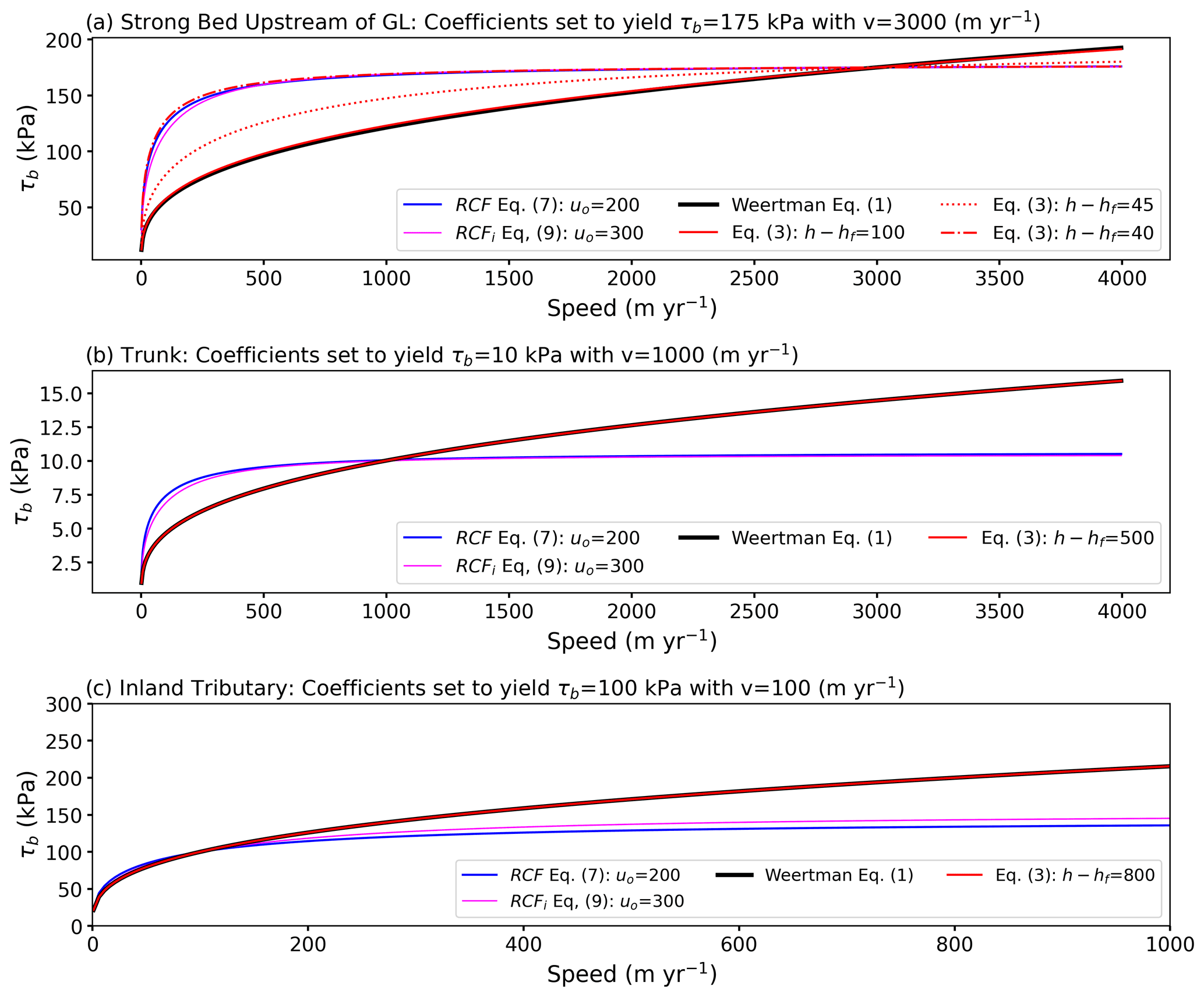
Figure 1Basal shear stress (τb) as a function of speed for conditions representative of flow (a) for the strong area upstream of the grounding line, (b) on the weak main trunk farther inland, and (c) with slow inland tributary flow. In each case, the sliding coefficients have been selected to produce the same speed basal resistance at a nominal reference speed. For the near-grounding-line case, the transition to full Coulomb friction begins at m (red dotted curve), with mixed conditions occurring at (red dot-dashed line).
The reason these plots largely reflect Weertman sliding is that the transition from Coulomb to Weertman conditions in Eq. (4) occurs at , with Eq. (3) producing a less abrupt transition at a similar value. Thus, if we assume ∼ 300 kPa to be the maximum expected value for τb with Coulomb friction, then the transition to Weertman sliding takes place at locations where the elevation is less than ∼ 67 m above flotation for α2=0.5. To illustrate the extent of the region where Coulomb conditions occur with these models, Fig. 2 shows contours of h−hf plotted over values of τb inferred as described in the Methods section. These contours indicate that Coulomb conditions only occur within about 10 km of the grounding line, which is consistent with the distances over which the assumption of perfect hydrological connectivity is likely valid (Asay-Davis et al., 2016).
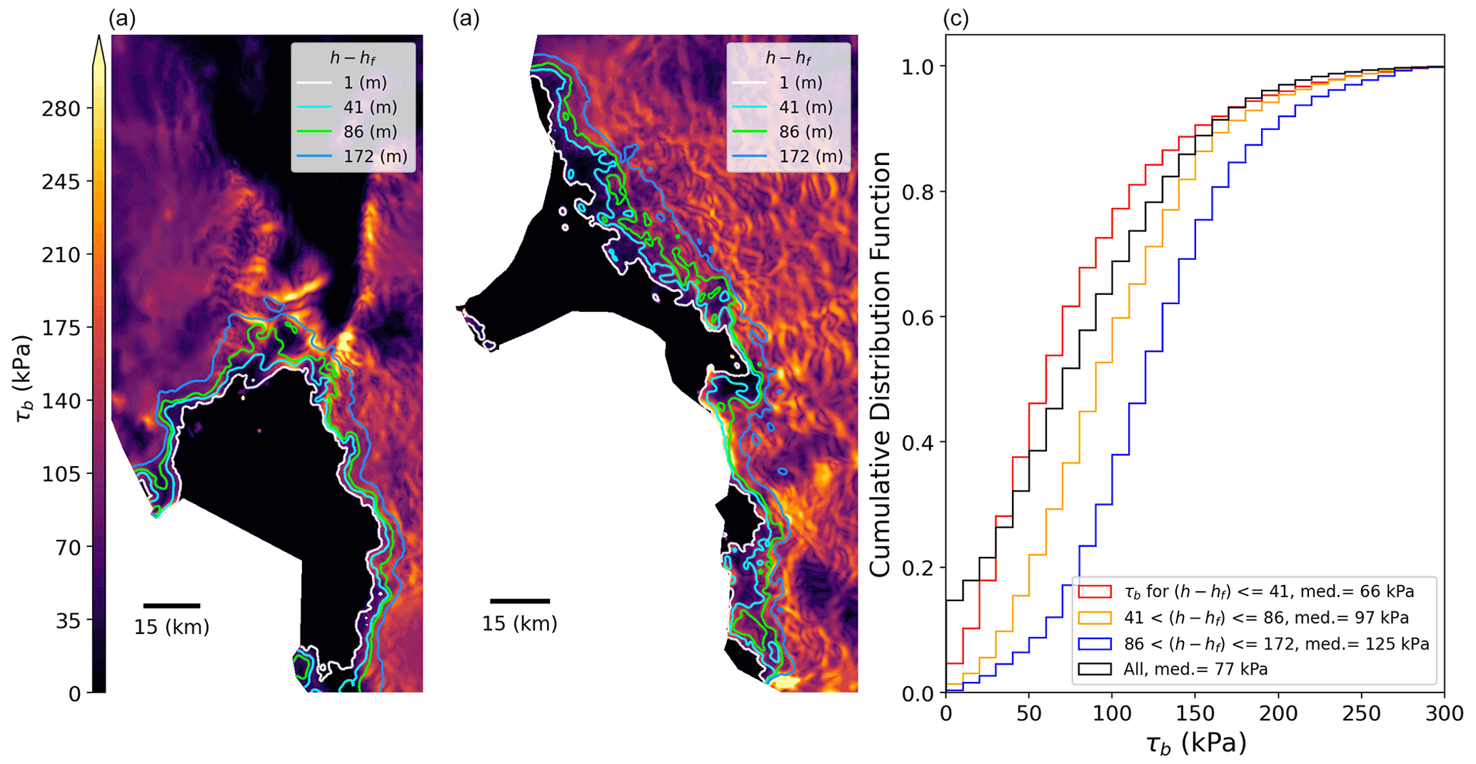
Figure 2Height-above-flotation (h−hf) contours plotted over inferred basal shear stress (τb from RCFi inversion) for (a) Pine Island and (b) Thwaites glaciers. (c) Cumulative distribution functions for τb for bands defined by h−hf. Note the contour values correspond to the value of hT used in our simulations.
Numerous boreholes indicate water pressures close to flotation and, thus, low (< 400 kPa) effective pressure (Luthi et al., 2002; Kamb, 2001) well away from the grounding line. The widespread presence of active subglacial lakes also suggests that low effective pressures are prevalent (Gray et al., 2005; Smith et al., 2009; Fricker et al., 2007; Bell, 2008). Recent hydrological models also support the presence of widespread areas of low effective pressure in the PIG and Thwaites Glacier basins (Dow, 2022; Hager et al., 2022). If this is the case, then Eqs. (3) and (4) indicate Coulomb conditions occur over a much broader area than that obtained by assuming basal water pressure to equal ocean pressure.
Weertman sliding can also include an effective pressure dependence. Initially based on laboratory measurements by Budd et al. (1979) and later modified by Fowler (1987), a modification of Weertman sliding that adds an explicit effective pressure dependence is given by
This equation is often applied with the effective pressure as given by Eq. (5), even at large distances from the grounding line, where the assumption is likely invalid (Yu et al., 2018). For the remainder of this article, we refer to Eq. (6) as Budd friction and Eq. (3) as Weertman sliding (or friction).
We know of no basal hydrological models for N that have been demonstrated to have sufficient accuracy to determine basal shear stress, leading to the often-used assumption given in Eq. (5). An alternate approach is to assume that effective pressures are low enough in regions of fast flow to produce Coulomb conditions. In this case, the observed speeds are assumed to determine the extent and type of basal friction, with the transition from Weertman to Coulomb behaviour occurring at some critical speed, uo. By subsuming the effective pressure into the sliding coefficient (β2), the form of the equation given by Schoof (2005) can be rewritten (Joughin et al., 2019) as
which we refer to as regularized Coulomb friction (RCF). In this case, the influence of N is determined implicitly in the solution for β2. Although this expression was derived for sliding-induced cavitation on hard beds (Schoof, 2005; Gagliardini et al., 2007), laboratory studies have shown that this form also applies to soft, deforming beds (Zoet and Iverson, 2020), albeit with a potentially different exponent. Thus, it may be reasonable to model friction with a single friction law (Minchew and Joughin, 2020). When modified as described below to allow near-grounding-line weakening and included in a model forced with observed elevation change, this friction model with m=3 most accurately reproduced the observed speedup of PIG over nearly 2 decades (Joughin et al., 2019). As indicated in Fig. 1, this equation produces Coulomb-like friction in regions of fast flow (|u|>uo) and Weertman-like conditions in areas of slower flow (|u|<uo; Fig. 1c). Another study indicated that PIG conditions are reproduced better with a power law using values of m in the range of 10–20, which produces a sensitivity of τb to speed that more closely resembles that of Eq. (7) than that of Weertman sliding (Gillet-Chaulet et al., 2016).
In addition to determining the transition from Weertman to Coulomb conditions, the sensitivity to h−hf for the assumed form of N used in Eqs. (3) and (4) causes the bed to weaken as the ice approaches flotation. This is a desirable effect, since it is unlikely that the basal traction goes from full strength to nothing precisely as the ice base goes from grounded to floating. To illustrate this point, Fig. 2c shows the cumulative distribution functions (CDFs) for values of τb inferred as described below for height-above-flotation-determined bands near the grounding line. The results show that in the band closest to the grounding line ( m), low τb values (median 66 kPa) are far more likely than ∼ 5–15 km farther inland ( m), where higher values of τb (medians of 97 and 125 kPa) are more prevalent. This characteristic is consistent with observations of a break in slope near the grounding line, indicating reduced driving and basal shear stresses (Fricker and Padman, 2006). These observations suggest that as the grounding line (zone) recedes inland to presently high-friction areas, some reduction in basal traction occurs.
Figure 3 shows the weakening as the surface elevation approaches flotation for Eqs. (3) and (4). The difference in these two formulations is that Eq. (3) combines Weertman and Coulomb basal resistance in parallel (Gudmundsson et al., 2023), which provides a smoother transition between the two friction types than the more abrupt transition when using Eq. (4).
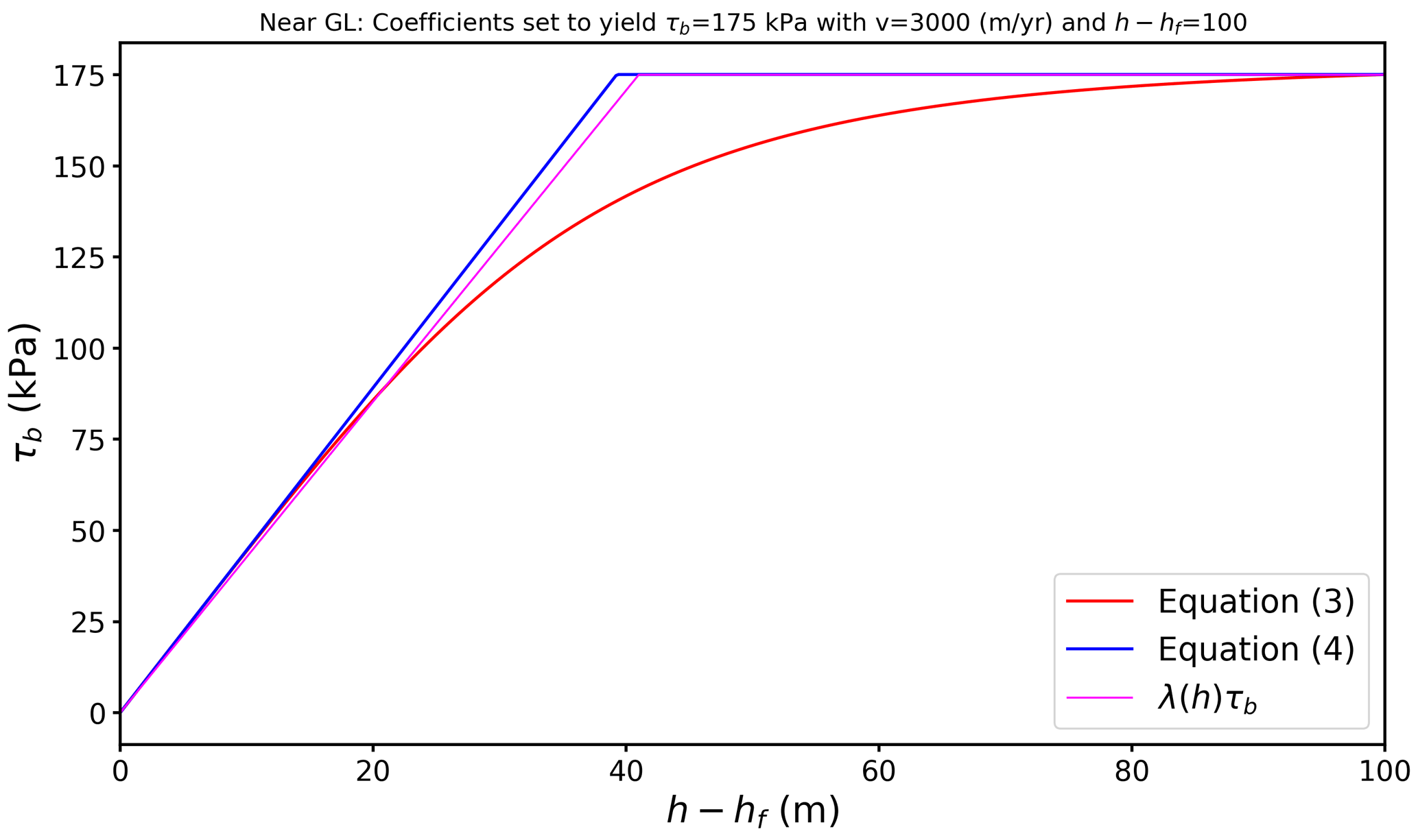
Figure 3Example of the decrease in basal resistance as ice approaches flotation for the different friction laws described in the text.
The Weertman and RCF models as parameterized above have no such weakening. To include this effect, Joughin et al. (2010) included a linear weakening of the bed that initiates once the height above flotation falls below some threshold, hT, which can be expressed as
where ho is the elevation at the start of the simulation. When used to scale Eqs. (1) or (7) (e.g. τb(h)=λ(h)τb), this function produces linear weakening as the surface elevation evolves with time similar to Eq. (4), as shown in Fig. 3. (Note that strengthening can occur in the rare instances where thickening occurs.) There is a critical difference, however, in that hT in Eq. (8) is fixed for all values of τb, whereas the elevation-dependent weakening in Eqs. (3) and (4) occurs with a spatially varying threshold determined by τb. The former assumes some critical threshold for effective pressure, which applies to a range of bed conditions. The latter assumes an effective pressure limit that depends on how much shear stress the bed can support. Both represent imperfect assumptions, and it is unclear which model is preferable in the absence of a better solution.
Earlier work suggested that a value of hT=41–46 m best reproduced PIG's response over the previous 2 decades (Joughin et al., 2019, 2021b) for the RCF model (Weertman sliding with m=3 produced the best results with hT=122–123 m). Figure 2, however, suggests the weakening may occur over a broader zone (see Fig. 2c). As a result, a major goal of the work presented here is to investigate the sensitivity of losses projected over centuries to this parameter. Here we perform experiments using Eq. (8) because it allows us to vary the amount of weakening so that we can study the resulting impact on ice loss. It also lets us separate the weakening behaviour from the friction model. Thus, many of the experiments described below are aimed at understanding the sensitivity of ice loss to the choice of hT.
Our numerical experiments are all conducted using a finite-element modelling package called icepack (Shapero et al., 2021). The remainder of this section describes the setup and initialization used to conduct the experiments described below.
3.1 Model
Our results are based on simulations using a basin-scale model of a coupled ice sheet–shelf system that was developed for earlier studies of PIG (Joughin et al., 2021a, b). The ice sheet modelling package, icepack (Shapero et al., 2021), used to construct this model is built around the finite-element analysis library Firedrake (Rathgeber et al., 2016), which includes an embedded symbolic language for specifying the differential equations to be solved. Both icepack and Firedrake are fully open-source and available through GitHub, as is the basin-scale model used for the work described herein.
The model solves the shallow-shelf equations (MacAyeal, 1989) on an unstructured finite-element mesh with triangular elements. The domain extent is fixed and the ice shelf front does not move, but the grounding line evolves freely. The mesh spacing is variable, with resolutions of a few hundred metres near the grounding lines and several kilometres in the deep interior (Fig. S1 in the Supplement). The model does not account for glacial isostatic adjustment, since this effect should be small at the 200-year timescales examined here (Larour et al., 2019). A typical 200-year simulation for the combined basins of the Pine Island and Thwaites glaciers takes a few days on a single CPU core with first-order elements and a time step of 0.01 years. Since everything is single-threaded, we can run ensembles in parallel on a multi-core machine over the same period.
Rather than using Eq. (7) to implement RCF, in icepack, it is numerically easier to solve for a different expression given by the following equation (Shapero et al., 2021):
We refer to the icepack version of regularized Coulomb friction as RCFi. Although Eqs. (7) and (9) appear substantially different in form, by adjusting the values of uo, they can produce nearly equivalent responses, as demonstrated in Fig. 1 (compare RCF and RCFi with values of uo equal to 200 and 300 m yr−1 in Fig. 1, respectively). For both RCFi and Weertman (Eq. 1 with m=3), we scale the basal shear stress by λ(h) using a range of hT.
We initialize the model by inverting for the basal friction law parameters (β2 for Weertman or RCFi, as appropriate) using standard methods implemented in icepack, with the amount of regularization determined through L-curve analysis (Hansen and O'Leary, 1993). The inversion procedure also solves for the Glen's flow law parameter, A, on the floating ice (Joughin et al., 2021a). For the grounded ice, the model determines A based on its temperature dependence (Cuffey and Paterson, 2010) using an earlier simulation for internal temperature (Joughin et al., 2009). Both A and β2 remain constant with time throughout each simulation.
For most of the experiments, we use a randomly generated ensemble of 30 melt distributions applied to the floating nodes (Joughin et al., 2021a), which are used to force 30 independent simulations. Unless otherwise noted, we present the results as the ensemble averages of these simulations. The melt distributions are selected such that approximately half produce peak melt at the grounding line, while the other half produce peak melt higher in the water column (see example profiles in Joughin et al., 2021a). At each time step (0.01 years), each melt distribution is re-normalized to produce a specified level of melt (e.g. 57 Gt yr−1). By contrast, many studies use a melt function parameterized by depth (e.g. Joughin et al., 2014; Gudmundsson et al., 2023; Jourdain et al., 2020; Yu et al., 2018; Barnes and Gudmundsson, 2022). In addition to our melt ensembles, we also conducted simulations with the depth-parameterized melt rates used in other recent studies (Gudmundsson et al., 2023; Yu et al., 2018; Barnes and Gudmundsson, 2022).
3.2 Initialization datasets
Our study area comprises the combined basins of PIG and Thwaites Glacier. Note that we treat Haynes Glacier as a branch of Thwaites Glacier so that all references hereafter to Thwaites apply to both glaciers. For the surface and bed elevations and thickness, we used the BedMachine version 3 dataset (Morlighem et al., 2020). We modified the bed elevations slightly to make them consistent with other data. First, we reduced bed elevations along some areas of the ice front to ensure they were floating, consistent with the assumed boundary condition. Second, we raised elevations for a few pockets in the interior to ensure that they were grounded. Finally, we reduced elevations downstream of the grounding line position of PIG that we inferred from 2014 TerraSAR-X speckled-tracked offsets (Joughin et al., 2016), which agrees well with the MEaSUREs version 2 grounding line (Rignot et al., 2014).
To invert for the friction coefficient, we used a velocity map assembled from three sources. First, we produced a map by processing all the Sentinel-1A/B data for the region collected from January 2019 to December 2020, which covered most of the model domain north of 78.7° S. Next, we filled gaps using data from the MEaSUREs Phase-Based Velocity Map (version 1) (Mouginot et al., 2019). Finally, for some of the slower, southernmost regions, where there were gaps or excessive noise in the MEaSUREs data, we used balance velocity data computed with a well-established algorithm (LeBrocq et al., 2006) constrained by RACMO 2.3 (Wessem et al., 2014) surface mass balance (SMB) data averaged from 1979 to 2022. Because most of the fast-moving areas are covered by the Sentinel-1 data, the final map is representative of the mean flow for 2019–2020.
For the surface mass balance (SMB), consistent with earlier studies (Joughin et al., 2021a, 2014), we used a map of SMB derived from airborne radar and ice cores (Medley et al., 2014), which does not vary with time. Using this SMB and initializing the model with the observed velocities, the combined system initially loses ice at a rate of 0.33 mm yr−1 sea level equivalent (s.l.e.), with PIG and Thwaites Glacier losing 0.17 and 0.16 , respectively. Note all values presented here are computed on a polar stereographic grid, which introduces area distortion. As a result, our estimated losses are biased low by ∼ 2.5 %.
Earlier work simulated the response of PIG to melt rate using hT=41 m (Joughin et al., 2021a), which is our preferred value, since it provides the best match to PIG's recent behaviour using RCFi (Joughin et al., 2019). The PIG record is, however, short (< 2 decades) relative to the periods over which sea level projections are required (centuries). To examine the sensitivity of simulated losses to the choice of hT and melt rate, we conducted further simulations with an expanded domain that also includes Thwaites Glacier.
Figure 4 shows the volume above flotation (VAF) losses for 200-year simulations with RCFi and our preferred value of hT (41 m), as well as for melt rates of 57, 75, 100, and 125 Gt yr−1 applied to each ice shelf (i.e. total melt for the domain is twice these values). For PIG the results agree well with those from earlier work (Joughin et al., 2021a), with small differences due to differences in the initial conditions and interactions with the adjacent Thwaites Basin. Thwaites Glacier and PIG produce similar losses throughout these simulations when forced with the same melt levels. Also shown are the combined VAF losses that would occur upon linear extrapolation of the current rates. The combined 200-year VAF losses are 73 % and 85 % of extrapolated current rates for melt rates of 57 and 75 Gt yr−1, respectively. With the higher melt rates, losses exceed the present rates by 7 %–28 %. As with the rest of the simulations described here, the results represent an average of 30 randomly selected melt profiles, each normalized to produce the prescribed amount of melt as described above.
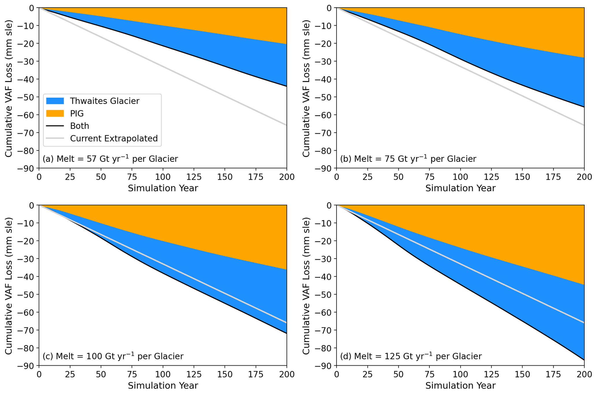
Figure 4Cumulative volume above flotation (VAF) losses for PIG and Thwaites Glacier simulated using RCFi for melt rates applied to each glacier's ice shelf of (a) 57, (b) 75, (c) 100, and (d) 125 Gt yr−1. For all simulations, hT=41 m. Also shown is the initial combined VAF loss rate based on the observed velocity linearly extrapolated over 200 years. All losses are subject to map-projection-related biases of a few percent.
Figure 5 shows the combined losses for both glaciers for the four values of hT that correspond to the height-above-flotation contours shown in Fig. 2. The simulations were conducted using both RCFi and Weertman sliding. For both types of friction, the VAF loss is strongly sensitive to the choice of hT. For the least melt (57 Gt yr−1), the largest value (hT=172 m) produces ∼ 40 % more loss than the smallest value (hT=1 m). At the highest melt rate (125 Gt yr−1), the corresponding difference is more than a factor of 2. The behaviour is similar for the Weertman cases, except that the sensitivity to hT is substantially lower at the lower end of the melt range. At the two lowest melt rates, nearly all the simulations produce less loss than extrapolation of the current rate. By contrast, the simulated losses exceed the extrapolated current rate, with the two highest melt rates for all but some of the cases with hT=1 m.
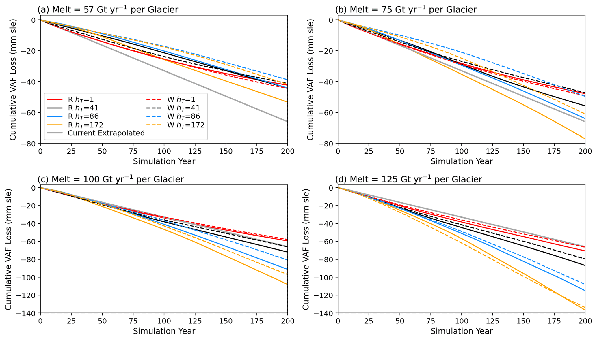
Figure 5Cumulative VAF loss for both glaciers simulated using both RCFi and Weertman sliding for several values of hT for melt applied to each glacier's ice shelf of (a) 57, (b) 75, (c) 100, and (d) 125 Gt yr−1. All losses are subject to map-projection-related biases of a few percent.
Figure 6 shows the annual loss rates for each glacier from the RCFi simulations. These results are averages of 30 simulations with differing melt distributions, so they tend to smooth out the variability of individual ensemble members as the grounding line retreats off basal highs (Joughin et al., 2021a). After a brief initial transient as the system equilibrates to the imposed melt, the VAF losses occur at relatively steady rates throughout most of the simulations. For Thwaites Glacier with the larger hT values, however, the annual rates of loss tend to increase substantially (∼ 2–3 times) throughout the simulation. At the most extreme (hT=172 m and 125 Gt yr−1 melt), the end-of-simulation loss rate for Thwaites Glacier is more than 5 times the present rate and more than twice the rate for PIG. As a result, much of the sensitivity to hT for the combined losses shown in Fig. 5 is attributable to Thwaites Glacier.
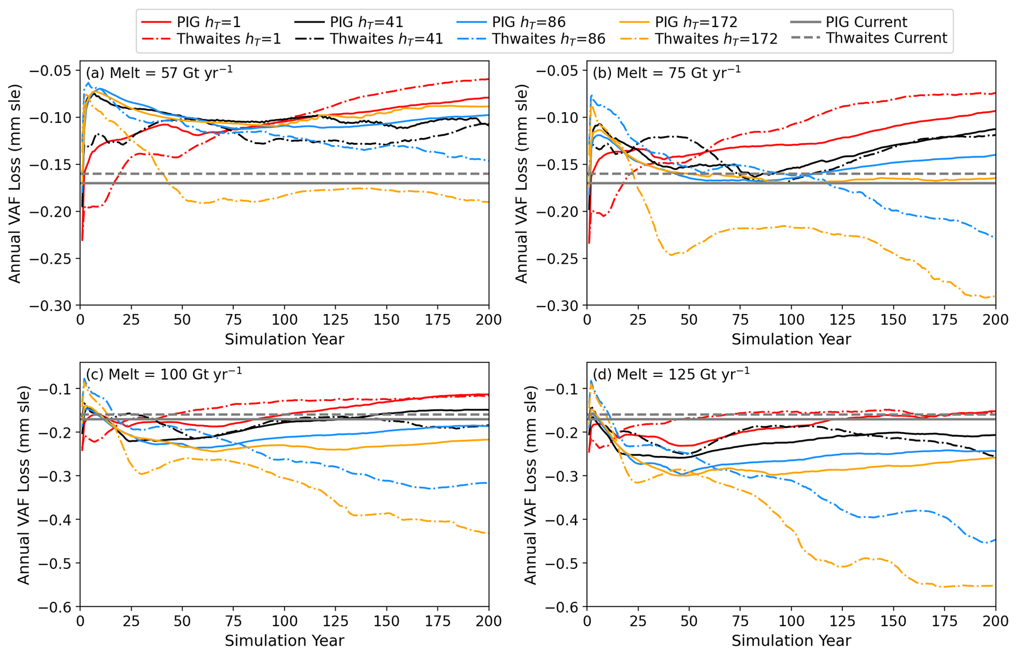
Figure 6Annual VAF loss for PIG and Thwaites Glacier simulated using RCFi with melt applied to each glacier's ice shelf of (a) 57, (b) 75, (c) 100, and (d) 125 Gt yr−1. The current rates based on velocities used to initialize the model are also shown. All losses are subject to map-projection-related biases of a few percent.
To examine the sensitivity to melt, Fig. 7 shows the 200-year losses as a function of the melt rate for the combined and individual glacier basins. To illustrate the sensitivity to the different spatial distributions of melt, this figure also shows the individual melt distribution ensemble members for the RCFi simulations. Linear fits to raw ensemble data (120 points for each fit) for both friction models are also shown. For the combined basin, the regressions show that the melt rate accounts for most of the variance (88 %–94 %), with the remaining variance due to the spatial distribution. The corresponding ranges are 81 %–97 % and 62 %–92 % for PIG and Thwaites Glacier, respectively. The sensitivity to melt increases with hT as indicated by the slopes for the combined RCFi responses, which vary from −0.21 to −0.61 over the range of hT values. The corresponding range of sensitivity is −0.24 to −0.51 for PIG and −0.18 to −0.71 for Thwaites Glacier. The results are similar for the Weertman cases, except that the sensitivity to hT is somewhat greater for PIG (−0.21 to −0.7 ). This increase in slope is largely due to the substantially lower losses for Weertman sliding at the lower end of the melt range.
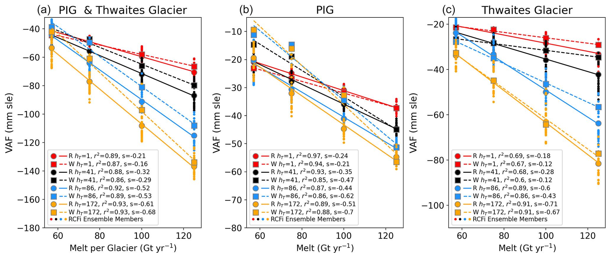
Figure 7Simulated 200-year VAF losses as a function of melt for (a) both glaciers, (b) PIG, and (c) Thwaites Glacier. Results are shown for several values of hT and both RCFi and Weertman sliding. Each result represents the average of an ensemble of 30 simulations with randomly generated melt distributions, which are shown only for the RCFi simulations. The lines show linear regressions to the ensemble data (4×30 points), with the corresponding slopes given in each legend. As such, the r2 values in the legend represent the proportion of the variance caused by the melt forcing.
To demonstrate their spatial distribution, Fig. 8 shows the VAF loss averaged over all 30 ensemble members at each level of melt for both the RCFi and Weertman simulations with hT=41 m. All the simulations have some thickening in the upper basin, which is likely due to the poorer quality of the velocity used to initialize the model there (i.e. speeds that are too slow). At the lower elevations, there is strong thinning of up to a few hundred metres that increases with melt level. At the higher melt values, the results from RCFi and Weertman are similar. At the lower melt levels, Weertman cases show some slight thickening near the PIG grounding line and less overall thinning, consistent with the results shown in Fig. 7. These results show PIG grounding line advance for the low-melt Weertman cases where thickening also occurred.
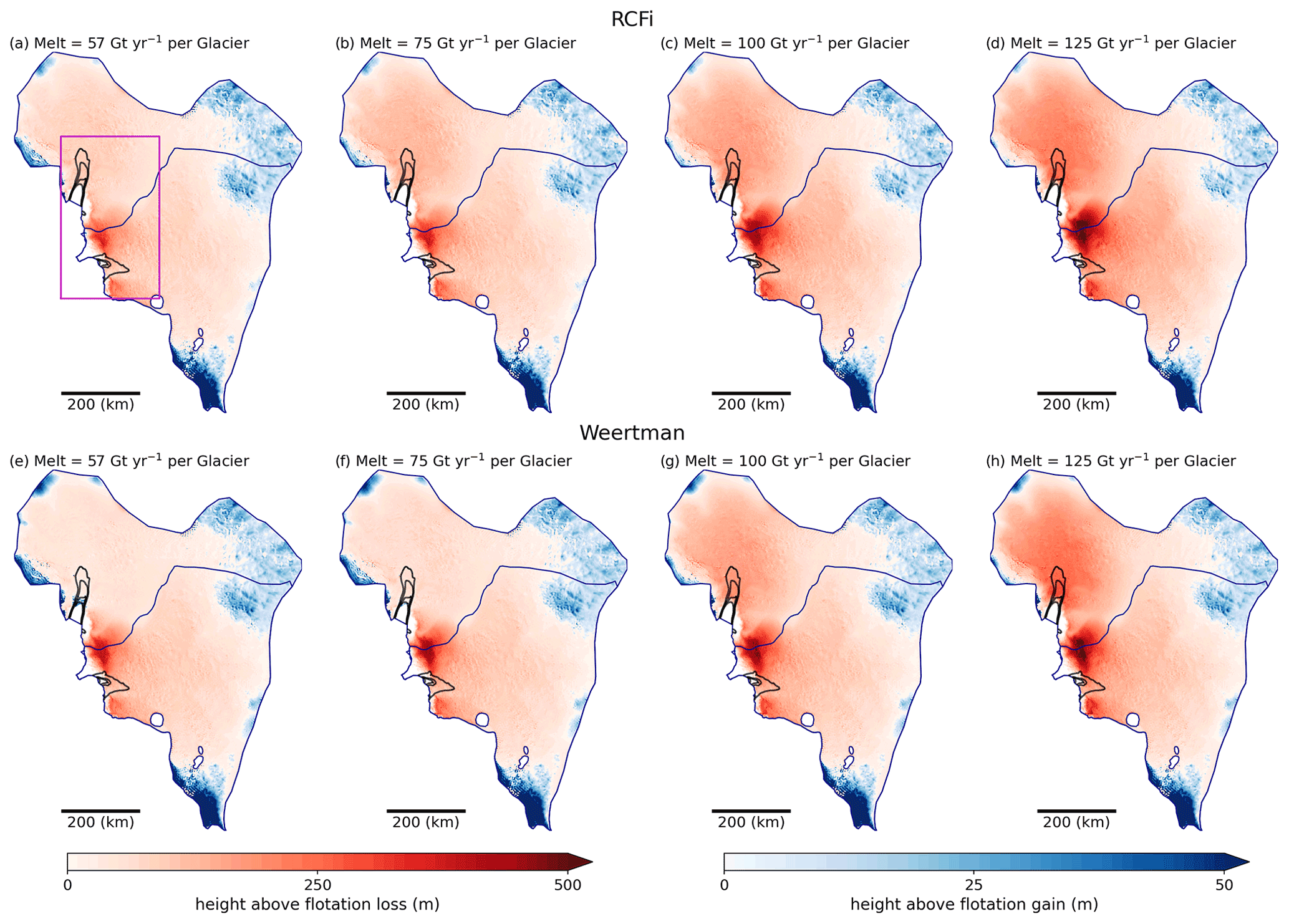
Figure 8Simulated 200-year VAF loss/gain for hT=41 m averaged over 30 ensemble members for RCFi with melt applied to each glacier of (a) 57, (b) 75, (c) 100, and (d) 125 Gt yr−1, as well as for Weertman sliding with melt of (e) 57, (f) 75, (g) 100, and (h) 125 Gt yr−1. Speed at intervals of 1000 m yr−1 is shown in black and basin boundaries are shown in blue. The magenta box in panel (a) indicates the area shown in more detail in Fig. 9.
Our simulations of the Pine Island and Thwaites glaciers reveal several important aspects of how projected contributions to sea level are influenced by the friction model, loss of traction upstream of the grounding line as ice thins (hT), and the melt rate.
5.1 Sensitivity to friction law
Overall, our results indicate that the choice of friction law yields relatively minor differences for the projected VAF losses (Fig. 7), except for the PIG cases with low melt. These differences are consistent with the PIG re-grounding seen in the low-melt simulations with Weertman sliding (Fig. 9e and f). As noted above, there are limited areas (ho<hT) where the bed can strengthen if thickening rather than thinning occurs. However, such thickening rarely occurs because the region near the grounding line nearly always tends to thin. For some Weertman cases, however, thickening and advance do occur for sufficiently low melt, which should be reinforced by thickening-induced strengthening of the bed near the grounding line. This would explain why the losses decline as hT increases for the low-melt Weertman cases on PIG, since the area subject to this type of strengthening expands. Whether this should remain a feature of our model is a subject for future research.
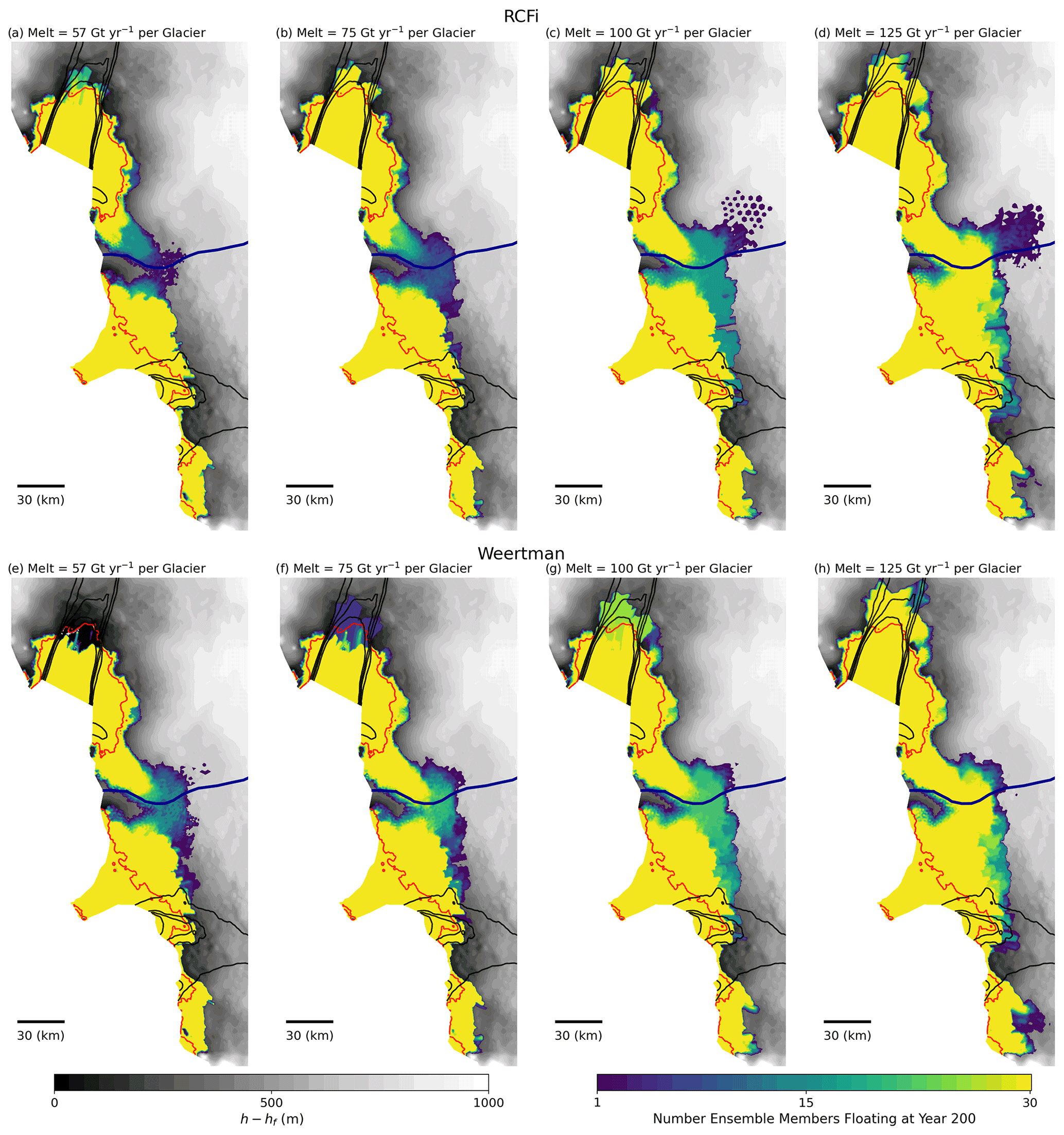
Figure 9The number of ensemble members' (colour) hT=41 m simulations at each point that are floating after 200 years simulated with RCFi for melt per glacier of (a) 57, (b) 75, (c) 100, and (d) 125 Gt yr−1, as well as with Weertman sliding for melt of (e) 57, (f) 75, (g) 100, and (h) 125 Gt yr−1. The speed at intervals of 1000 m yr−1 is shown in black.
On Thwaites Glacier, all the simulations result in retreat, and the RCFi and Weertman simulations produce roughly similar results in terms of grounding line retreat (Fig. 9) and VAF loss (Figs. 7 and 8). Overall, the grounding line retreat is more variable for Thwaites Glacier (blue-green areas in Fig. 9). This variability likely occurs because approximately half the ensemble members tend to produce shallower melt distributions that shift a larger portion of the melt to the eastern shelf, which should enhance retreat along the eastern portion of the grounding line. Thus, while the choice of the form of the frictional law makes a relatively small difference (< 20 %) in general, the friction models cannot be treated interchangeably, since in some circumstances, the differences can be large (> 50 %) and unpredictable, as in the low-melt PIG simulations. Since RCFi is better able to reproduce recent behaviour on PIG and because Weertman friction can cause grounding line advance (Fig. 9) that is inconsistent with current observations, RCFi seems preferable for studies in which only one type of friction is used.
Several studies have compared Weertman sliding with the friction laws expressed in Eqs. (3) and (4) (Gudmundsson et al., 2023; Barnes and Gudmundsson, 2022; Nias et al., 2016). Comparisons of our work with these studies are hindered by the fact that while the friction laws represented by these equations are often referred to as regularized Coulomb friction, they produce Coulomb friction for only a small fraction of the bed (< 1 % of the domain) near the grounding line (h−hf < ∼ 86 m in Fig. 2) so that the vast majority of the basin is subject to Weertman sliding. By contrast, RCFi applies Coulomb conditions to the full extent of the fast-moving regions (∼ 11 % of the domain). A further complicating factor is the extent to which Eqs. (3) and (4) differ from Weertman due to Coulomb behaviour (i.e. the dependence of τb on speed) versus their dependence on effective pressure (i.e. reduction in traction as flotation is approached). Moreover, such an effective-pressure-dependent reduction is not limited to Coulomb friction and such a dependence can be included in a Weertman model, as is the case for Eq. (6).
An advantage of our approach is that we can evaluate how the friction law and the weakening above the grounding line individually affect ice loss. As the latter appears to play a larger role, we defer further comparison to the discussion below, where we examine the sensitivity of our results to hT.
5.2 Sensitivity to weakening as ice approaches flotation
Figure 2c indicates that the area near the grounding line ( m) is substantially weaker than the area immediately above it ( m), which suggests the need for a mechanism to reduce basal traction as the ice column evolves toward flotation. This reduction can be accomplished either explicitly through Eq. (8) or implicitly through the dependence on effective pressure in Eqs. (3) and (4). All of our simulations use the explicit approach.
The results shown in Figs. 5–7 indicate a strong sensitivity to the rate at which traction above the grounding line is reduced in our simulations, as parameterized via hT. Larger values of hT tend to produce more loss at the same melt level due to the additional loss of basal traction as the ice thins. An exception occurs for PIG with RCFi, where at low melt values, the losses are nearly the same across the full range of hT. An earlier analysis of PIG indicated that while loss of traction acts to speed up the glacier, much of this effect is counterbalanced by the evolution of the surface, which reduces the driving stress near the grounding line (Joughin et al., 2019). In most cases the loss of basal traction appears to prevail, leading to an overall speedup. At low melt rates on PIG, however, these two competing effects appear to roughly balance each other out over the full range of hT. Thwaites Glacier's losses are far more sensitive to hT, with the minimum and maximum values producing differences of ∼ 60 % at the low end of the melt range and of up to a factor of 2.8 at the upper end of the range. This enhanced sensitivity is likely due to the glacier's weak shelf, which is less able to produce additional buttressing as it speeds up to help compensate for the greater loss of basal traction due to high melt with a large value of hT.
As Fig. 3 indicates, the loss of traction near the grounding line as the ice approaches flotation is similar in form for Eqs. (3), (4), and (8). The key difference is that for our simulations, the linear reduction in traction is determined by a spatially invariant threshold (hT). The way Eqs. (3) and (4) are formulated means that they effectively have similar thresholds, except that they vary spatially based on the basal shear stress at each point. These differences tend to make direct comparisons difficult. One way to obtain a rough equivalency is to determine the value of hT that yields equivalent area-integrated traction subject to reduction via the effective pressure dependency in Eq. (4) for a given value of α2.
Barnes and Gudmundsson (2022) conducted simulations using α2 values of 0.25, 0.5, and 0.75 in Eq. (3), which roughly translate to hT values of 57, 27, and 17 m, respectively, using the method just described. These values bracket our preferred value of 41 m, which indicates that this choice of hT is consistent with the range of values used by the latter authors as well as values used in other studies. In the study by Barnes and Gudmundsson (2022), several 120-year simulations were conducted for a domain that also included the Smith, Pope, and Kohler glaciers. When they used the friction model described by Eq. (3), the results were 20 % and 38 % greater relative to Weertman sliding (α2→∞) for α2 values of 0.5 (hT∼27 m) and 0.25 (hT∼57 m), respectively. Over the same period using Weertman sliding scaled by λ(hT) with hT=41 m, we obtained results that were 23 % greater than with hT=1 m (Weertman with effectively no weakening). Given the differences in the models and domains, our results are in good agreement, suggesting that most of the additional losses in the Barnes and Gudmundsson (2022) results are due to the reduction in basal traction as the effective pressure declines rather than due to the transition to Coulomb conditions in the region near the grounding line.
The fact that our empirically derived value of hT agrees well with roughly equivalent values determined from consideration of effective pressure suggests that both types of models tend to reduce basal traction at rates that are of approximately the right magnitude. While we cannot completely discount the results from the larger values of hT used in our simulations, they likely produce losses that are larger than can be expected.
Consistent with the other work cited above, the results presented herein suggest that models should include some type of reduction in basal traction as flotation is approached, irrespective of the actual friction type (e.g. Weertman or Coulomb). Less clear is how such weakening should be applied. While empirical in nature, Eq. (8) has demonstrated a reasonable ability to reproduce the observed behaviour (Joughin et al., 2019). There is no reason, however, that α2 in Eqs. (3) and (4) cannot be selected through a procedure like that used to derive our preferred value of hT. On the other hand, Eq. (8) can easily be modified to have a spatial variable hT that depends on effective pressure in a similar manner to Eqs. (3) and (4), which would allow the traction reduction to be decoupled from the form of the basal friction law. The best combination of these concepts is a subject for future research.
Our best estimate for hT is based solely on the response of PIG over a decade and a half. While it is likely that other glaciers can be modelled well with a value of hT of similar magnitude, further work is needed to establish the best value for other regions. Our results, however, do establish that the choice of hT can have a substantial effect on projected losses, as is the case for α2 (Barnes and Gudmundsson, 2022).
As the ice evolves in areas away from the grounding line, the driving stress increases in some areas and decreases in others. The extent to which the friction law parameters are static, as is often assumed, is unclear, as is whether they should rather co-evolve with the driving stress or other changes in ice sheet geometry that influence effective pressure. Lacking a good model to vary the friction as the surface evolves, except near the grounding line, many models, including ours, allow basal traction in the interior only to respond to variations in speed (e.g. Seroussi et al., 2020). Budd friction with effective pressure determined by Eq. (6) is an exception in that the basal traction is reduced over the entire model domain in direct response to thinning. When using this type of friction, projected losses can more than double (Yu et al., 2018; Barnes and Gudmundsson, 2022). With q=3 and m=3 in Eq. (6), the result is equivalent to Weertman friction with unbounded hT (i.e. basal traction declines linearly with reductions in h−hf). The assumption, however, that a hydrologic connection to the ocean exists over the full domain, such that the water pressure is equal to ocean pressure, is not well supported by borehole observations of water pressure (Luthi et al., 2002; Kamb, 2001) and the widespread presence of subglacial lakes (Gray et al., 2005; Smith et al., 2009; Fricker et al., 2007; Bell, 2008) or by pertinent models (Dow, 2022; Hager et al., 2022). We suggest that any law that relies solely on the local height above flotation to govern changes in effective pressure (e.g. Eq. 6) and, thus, basal friction over the entire domain is likely oversimplified and incorrect. Other factors, such as the surface slope, should influence the basal hydrological system that determines the effective pressure. As a result, care should be taken when interpreting results that employ Budd friction (Eq. 7) in the absence of a more accurate means of determining the effective pressure.
5.3 Sensitivity to melt
Our results indicate that the combined and individual losses for PIG and Thwaites Glacier increase linearly with melt (Fig. 7), consistent with similar work for just PIG (Joughin et al., 2021a). For PIG, the linear fits to the 120 ensemble members for each friction model (30 melt distributions for each of four melt levels) indicate that the spatiotemporally averaged melt has a far greater effect on ice loss (r2=0.86–0.97) than either the spatial or temporal variation of the melt, consistent with an earlier study that simulated just the PIG Basin (Joughin et al., 2021a). The PIG ice shelf provides substantial backstress (Gudmundsson et al., 2023). As a result, increasing the discharge to the shelf provides more backstress (faster flow and thicker ice), which acts as a negative feedback to the speed. Greater melting weakens this response, allowing greater discharge. For Thwaites Glacier, the sensitivity to melt is weaker for lower values of hT, with less of the variance being explained by the trend (r2=0.6–0.69). Thwaites Glacier is not nearly as well buttressed by its ice shelf as PIG (Gudmundsson et al., 2023), so the flow is less sensitive to melt-induced thinning of the shelf at low values of hT, which is consistent with an earlier sensitivity study (Nias et al., 2016). Moreover, Thwaites Glacier feeds a broad weak shelf with a shallow draft and narrow, deep pockets that provide some buttressing (Gudmundsson et al., 2023). As mentioned above, some of the shallower melt distributions will concentrate more of the melt at the eastern shelf to yield more variable results.
We used a fixed melt level throughout each simulation. In other work on PIG, however, similar simulations with periodic melt forcing (periods of decades to centuries), linear melt trends, and steady melt all produced virtually the same losses in cases where the long-term average melt was the same (Joughin et al., 2021a). This finding might appear to contradict other work suggesting melt-rate variability around a constant long-term average rate can affect overall VAF loss (Robel et al., 2019; Hoffman et al., 2019). These studies, however, examine fluctuations in melt rate rather the volume, which is a function of both the melt rate and the shelf geometry. For example, a constant melt rate will lead to an increasing melt volume as the shelf area expands with ungrounding. Thus, we speculate that if these earlier results were recast as functions of melt volume, they would then exhibit a similar linearity with melt volume as our results. While we are not well positioned to repeat these prior experiments, we can examine whether such linearity holds for a melt volume that freely evolves when driven by fixed depth-dependent melt-rate parameterizations. To do so, we conducted additional experiments using the depth-parameterized functions used in other studies (Barnes and Gudmundsson, 2022; Gudmundsson et al., 2023; Yu et al., 2018), which allow the melt to vary freely as the shelf evolves. These simplified melt functions (Fig. S2 in the Supplement) are meant to crudely emulate a plume originating in a warm bottom layer (< 500–1000 m) with high melt rates (40–160 m yr−1) that rises through a linear melt gradient approximating the thermocline at middle depths, above which the plume loses all ability to melt ice.
Figure 10 shows the results using these 10 depth-parameterized melt rates, which produce an average melt per glacier ranging from 36 to 389 Gt yr−1, with melt on Thwaites Glacier of up to 549 Gt yr−1. Linear regressions to the results from these simulations produce r2 values of 0.96 or greater, except for one case on Thwaites Glacier (r2=0.9 for hT=1). The independently determined regressions from our constant-melt ensembles all fit nearly as well (–0.98). These results indicate that the linear increases with steady melt evident in Fig. 7 also apply when the melt freely evolves with the shelf geometry. We note that the regressions to the depth-parameterized melt rates typically yield higher r2 values (Fig. 10) than the regressions to the constant-melt ensemble data (Fig. 7), which may be a statistical quirk. The better fits for the depth-parameterized functions, however, may reflect the fact that our melt ensembles employ a wider range of depth variation. For example, all the depth-parameterized melt functions produce maximum melt in the bottom part of the water column near the grounding line. By contrast, half of the ensemble distributions produce maximum melt higher in the water column, as some models suggest should be the case (Favier et al., 2019)
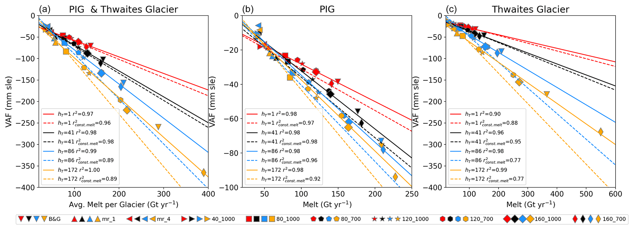
Figure 10Simulated 200-year VAF losses as a function using depth-parameterized melt functions for (a) both glaciers, (b) PIG, and (c) Thwaites Glacier with RCFi. Results are shown for several values of hT. The solid lines show the linear regressions to the plotted points, and the dashed lines are those computed from the RCFi ensemble data shown in Fig. 7. The values show the fraction of variance that the constant-melt regression parameters explain for the depth-parameterized melt-function simulations.
Both our ensembles and the depth-parameterized melt simulations reveal that ice losses increase linearly with melt. Although we used a single model, the ISMIP6 suite of models yields similar results (Seroussi et al., 2020), with a linear regression of sea level rise on melt yielding r2=0.93 for the Amundsen Sea Embayment (Joughin et al., 2021a). Based on a similar assumption of linearity, Levermann et al. (2020) characterized sea level uncertainty from Antarctica by generating large ensemble estimates based on a more limited number of runs from ISMIP6. The linear response to melt shown in Figs. 7 and 10 supports the use of their approach, which may help limit the computational burden for large ensemble projections.
Given that shelf-wide total melt is a robust predictor of sea level rise contributions, future studies should include total melt values in addition to other descriptors of melt (e.g. average melt rates or melt parameterizations) to facilitate comparison with other studies, as discussed above. For example, plotting results from multiple studies as shown in Fig. 10 would help differentiate the cases where different models produce results consistent with the level of melt forcing (e.g. the results lie along a linear regression line with high r2 near 1) from those in which the differences are due to some other aspect of the model (e.g. results are not explained well by a linear regression to melt). For example, the fact that melt is a strong predictor of loss in the Amundsen Sea Embayment for the suite of ISMIP6 models (Seroussi et al., 2020) suggests that much of the difference between models in this region may be due to how they treat melt as opposed to differences in their treatment of ice dynamics.
Our use of prescribed rather than freely evolving melt rates does not necessarily emulate natural processes. It does, however, provide a controlled means to evaluate the response of a coupled ice sheet–ice shelf system to melt forcing. The resulting regressions reliably predict the VAF loss in cases where the total melt can be determined (e.g. dashed curves in Fig. 10).
While we used a constant melt forcing, a melt history supplied by any methods that can estimate total melt for a given cavity geometry (e.g. offline ocean model) could also be used. Removing the details of the spatial distribution of melt may allow the use of simpler, more loosely coupled models that only need to determine the total melt at infrequent intervals, so long as they track the long-term melt trend.
5.4 PIG and Thwaites Glacier outlook
Our simulations are not projections, since they are not tied to climate forcings. Nor do they include factors unrelated to ocean melt, such as increased accumulation as atmospheric temperatures rise (Donat-Magnin et al., 2021), loss of ice shelf area, or glacial isostatic adjustment (Larour et al., 2019). Nonetheless, they do provide some sense of how much these glaciers will contribute to sea level rise over the next 2 centuries in response to basal melt.
Prior estimates for PIG melt range from 76 to 101 Gt yr−1 (Rignot et al., 2013; Depoorter et al., 2013; Shean et al., 2019; Adusumilli et al., 2020), but these estimates cover an area substantially larger than our domain. A recent melt estimate from remote sensing that covers an area similar to our model domain is 67 Gt yr−1, with substantial interannual variability (Joughin et al., 2021a). This value lies between our 57 and 75 Gt yr−1 simulations, both of which produce future losses lower than the present rate. The current rates, however, include speedup due to recent ice shelf loss, which is expected to decline as the system adjusts to the new geometry. Our 100 and 125 Gt yr−1 simulations produce long-term average losses greater than present for PIG with hT≥41 m.
Recent simulations of water temperatures with regional-scale ocean models forced with climate model output indicate that melt rates on PIG will increase by ∼ 5–8 m yr−1 (Jourdain et al., 2022), which is equivalent to 21 Gt yr−1 by 2100 for the current ice shelf geometry. If there is a similar increase for the next century, then our 125 Gt yr−1 estimate would still exceed the 2-century average. This analysis, however, does not allow for increases in ice shelf area (Fig. 9), which also influence the melt rate. Neglecting the expansion of the ice shelf may not have a big impact on results for PIG. A coupled ice–ocean model produces a relatively steady melt rate of ∼ 150 Gt yr−1 for warm conditions (base of the thermocline at 600 m) through a 120-year simulation in which the glacier has a total VAF loss of 50 mm s.l.e. (Bett et al., 2023). Our simulations with depth-parameterized melt rates do allow the melt to increase as the ice shelf area expands, though not necessarily in a way that realistically accounts for ocean circulation. The most aggressive melt parameterization (see 160_700 in Fig. S2) for PIG yielded an average melt rate of 182 Gt yr−1. If we take the corresponding VAF loss as an upper bound, then the maximum 2-century melt-driven VAF loss from PIG is 63 mm s.l.e. (Fig. 10; hT=41 m), 24 mm s.l.e. of which occurs over the first century of the simulation.
The evolution of the Thwaites Ice Shelf's cavity is more complex because in advanced stages of grounding line retreat, it broadens and deepens, providing a much greater area exposed to high melt rates at depth. Based on an ocean model with warm conditions used by Bett et al. (2023), melt increases from ∼46 Gt yr−1 for the current geometry to ∼ 220 Gt yr−1 when the VAF loss reaches ∼ 40 mm s.l.e. Although their model loses mass much faster than ours due to its treatment of the ice dynamics, the melt rates the ocean model produces at a particular VAF loss should not depend heavily on the time taken to reach that state if the temperature forcing is steady, as in this case. Assuming a linear increase, these rates imply an average melt rate of ∼ 133 Gt yr−1. For comparison, our 125 Gt yr−1 melt rate produces a VAF loss of 39 mm s.l.e. (hT=41 m). Thus, for the warm conditions they used, our simulation suggests losses of ∼ 40 mm s.l.e. over the next 200 years. As the cavity beneath the Thwaites Ice Shelf increases in response to greater losses, the melt rates could eventually reach 600 Gt yr−1 (Bett et al., 2023), indicating that much larger losses may be likely in the 23rd century and beyond. For comparison, the most aggressively parameterized melt-rate function for Thwaites Ice Shelf produces an average melt rate of 151 Gt yr−1 (hT=41 m; see B&G in Fig. 10c), which yields a VAF loss of 46 mm s.l.e. (Fig. 10). (Note that while 160_700 yields less melt, it produces a slightly larger loss for Thwaites Glacier.) Thus, melt-driven losses for Thwaites Glacier are likely to remain relatively moderate (< 50 mm s.l.e.) over the next 2 centuries with our preferred value of hT (41 m), which is comparable to PIG. After 200 years, however, as melt rates increase, losses should accelerate rapidly (Joughin et al., 2014). If it turns out that larger values of hT should be used in place of our preferred value, then the period of rapid losses for Thwaites Glacier could occur earlier and losses could greatly exceed those from PIG (Fig. 10).
We have conducted several numerical simulations for the Pine Island and Thwaites glaciers to understand how their projected contributions to sea level over the next 2 centuries are affected by the amount of melt and the choice of friction law. In most cases, the choice of friction law makes little difference if the same loss of basal traction occurs as the region near the grounding line approaches flotation. Our preferred value (hT=41 m) produces ∼ 20 % more loss than the cases in which there is an abrupt transition from full friction to no friction as the ice column becomes afloat (hT=1 m). The value of hT=41 m is roughly consistent with the degree of weakening introduced by other regularized Coulomb friction laws. Our results indicate, however, that the weakening itself introduced by these friction laws has a far more significant effect than the introduction of Coulomb rather than Weertman conditions over a small (< 1 %) fraction of the domain. The possibility remains that sea level contributions could be much larger (> 2 times) if a value of hT substantially larger than our preferred value is found to be more appropriate.
Our results indicate that irrespective of the choice of hT, losses are a linear function of the total melt averaged over the full simulation period. This linearity holds for simulations with both constant melt and freely evolving depth-parameterized melt. The spatial distribution of the melt has little effect on overall VAF loss. Each glacier, however, has a different sensitivity to melt. With its better-buttressed ice shelf, PIG yields about 50 % more VAF loss for each incremental increase in the melt than Thwaites Glacier. Thus, despite the complexity of the non-linear system, 200-year simulated losses from the glaciers are reliably predicted solely by the spatiotemporally averaged melt rate.
While we cannot account for other factors that might increase ice loss, such as full ice shelf breakup (MacAyeal et al., 2003) or partial shelf loss (Joughin et al., 2021b), our results suggest that melt-driven losses from PIG and Thwaites Glacier over the next 2 centuries may not exceed 10 cm. At 2 centuries out, however, both glaciers will have lost a substantial amount of ice and will be primed for much more rapid loss if melt rates do not subside.
The original BedMachine bed and surface elevation and thickness data (https://doi.org/10.5067/FPSU0V1MWUB6, Morlighem, 2022) as well as the MEaSUREs Phase-Based Antarctica Ice Velocity Map V001 (https://doi.org/10.5067/9T4EPQXTJYW9, Mouginot et al., 2017) are available at NSIDC. To allow for any updates that may occur during the revision process, we defer the permanent archiving of all other data used to constrain the model until final acceptance. The basin-scale model, all data, and model inputs are freely available at Dryad (https://doi.org/10.5061/dryad.7sqv9s50x, Joughin et al., 2024).
Icepack is available at https://icepack.github.io (last access: 20 July 2023, commit 0c17259979b1e595fdfcccb53bdc6f3d033755c4) and https://doi.org/10.5281/zenodo.7897023 (Shapero et al., 2023). The basin-scale model and supporting code are available at https://github.com/fastice/icesheetModels (last access: 4 December 2023, commit 5c94064) and https://github.com/fastice/modelfunc (last access: 9 August 2023, commit 904c8a9) and https://doi.org/10.5061/dryad.7sqv9s50x (Joughin et al., 2023).
The supplement related to this article is available online at: https://doi.org/10.5194/tc-18-2583-2024-supplement.
IJ conceived the ideas with support from PD. The basin-scale model was written by IJ, and he performed the model runs and analysis of the results with input from PD and DS. DS wrote the icepack modelling package and provided guidance on its use. All authors contributed to the production of the final manuscript.
The contact author has declared that none of the authors has any competing interests.
Publisher's note: Copernicus Publications remains neutral with regard to jurisdictional claims made in the text, published maps, institutional affiliations, or any other geographical representation in this paper. While Copernicus Publications makes every effort to include appropriate place names, the final responsibility lies with the authors.
Ian Joughin and Daniel Shapero were funded by the National Aeronautics and Space Administration (NASA) and the National Science Foundation (NSF), and Pierre Dutrieux was funded by the National Environment Research Council (NERC).
We acknowledge data contributions from the EU/ESA Copernicus Sentinel-1A/B missions, Mathieu Morlighem (BedMachine), Ian Howat (REMA data included with BedMachine), E. Rignot (MEaSUREs Velocities), and Brooke Medley (SMB Map). Balance velocities were produced using code supplied by Jonathan Bamber and developed by Anne LeBrocq, which was constrained by RACMO 2.3 data produced by the Institute for Marine and Atmospheric Research Utrecht (IMAU). Comments by Mai Maki, Tyler Pelle, an anonymous reviewer, and Felicity McCormack (editor) led to improvements in the final manuscript.
This research has been supported by the National Aeronautics and Space Administration (grant no. 80NSSC20K0954), the National Science Foundation (grant no. OAC-1835321), and the National Centre for Earth Observation.
This paper was edited by Felicity McCormack and reviewed by Tyler Pelle and one anonymous referee.
Adusumilli, S., Fricker, H. A., Medley, B., Padman, L., and Siegfried, M. R.: Interannual variations in meltwater input to the Southern Ocean from Antarctic ice shelves, Nat. Geosci., 13, 616–620, https://doi.org/10.1038/s41561-020-0616-z, 2020.
Asay-Davis, X. S., Cornford, S. L., Durand, G., Galton-Fenzi, B. K., Gladstone, R. M., Gudmundsson, G. H., Hattermann, T., Holland, D. M., Holland, D., Holland, P. R., Martin, D. F., Mathiot, P., Pattyn, F., and Seroussi, H.: Experimental design for three interrelated marine ice sheet and ocean model intercomparison projects: MISMIP v.3 (MISMIP+), ISOMIP v.2 (ISOMIP+) and MISOMIP v.1 (MISOMIP1), Geosci. Model Dev., 9, 2471–2497, https://doi.org/10.5194/gmd-9-2471-2016, 2016.
Barnes, J. M. and Gudmundsson, G. H.: The predictive power of ice sheet models and the regional sensitivity of ice loss to basal sliding parameterisations: a case study of Pine Island and Thwaites glaciers, West Antarctica, The Cryosphere, 16, 4291–4304, https://doi.org/10.5194/tc-16-4291-2022, 2022.
Bell, R. E.: The role of subglacial water in ice-sheet mass balance, Nat. Geosci., 1, 297–304, https://doi.org/10.1038/ngeo186, 2008.
Bett, D. T., Bradley, A. T., Williams, C. R., Holland, P. R., Arthern, R. J., and Goldberg, D. N.: Coupled ice/ocean interactions during the future retreat of West Antarctic ice streams, The Cryosphere Discuss. [preprint], https://doi.org/10.5194/tc-2023-77, in review, 2023.
Blankenship, D. D., Bentley, C. R., Rooney, S. T., and Alley, R. B.: Till beneath ice stream B: 1. Properties derived from seismic travel times, J. Geophys. Res.-Sol. Ea., 92, 8903–8911, https://doi.org/10.1029/jb092ib09p08903, 1987.
Budd, W. F., Keage, P. L., and Blundy, N. A.: Empirical Studies of Ice Sliding, J. Glaciol., 23, 157–170, https://doi.org/10.1017/s0022143000029804, 1979.
Cuffey, K. M. and Paterson, W.: The Physics of Glaciers, 4th edn., Elsevier, ISBN 9780123694614, 2010.
Depoorter, M. A., Bamber, J. L., Griggs, J. A., Lenaerts, J. T. M., Ligtenberg, S. R. M., van den Broeke, M. R., and Moholdt, G.: Calving fluxes and basal melt rates of Antarctic ice shelves, Nature, 502, 89–92, https://doi.org/10.1038/nature12567, 2013.
Donat-Magnin, M., Jourdain, N. C., Kittel, C., Agosta, C., Amory, C., Gallée, H., Krinner, G., and Chekki, M.: Future surface mass balance and surface melt in the Amundsen sector of the West Antarctic Ice Sheet, The Cryosphere, 15, 571–593, https://doi.org/10.5194/tc-15-571-2021, 2021.
Dow, C. F.: The role of subglacial hydrology in Antarctic ice sheet dynamics and stability: a modelling perspective, Ann. Glaciol., 63, 49–54, https://doi.org/10.1017/aog.2023.9, 2022.
Dutrieux, P., Rydt, J. D., Jenkins, A., Holland, P. R., Ha, H. K., Lee, S. H., Steig, E. J., Ding, Q., Abrahamsen, E. P., and Schroeder, M.: Strong sensitivity of Pine Island ice-shelf melting to climatic variability, Science, 343, 174–178, https://doi.org/10.1126/science.1244341, 2014.
Favier, L., Durand, G., Cornford, S. L., Gudmundsson, G. H., Gagliardini, O., Gillet-Chaulet, F., Zwinger, T., Payne, A. J., and Brocq, A. M. L.: Retreat of Pine Island Glacier controlled by marine ice-sheet instability, Nat. Clim. Change, 4, 117–121, https://doi.org/10.1038/nclimate2094, 2014.
Favier, L., Jourdain, N. C., Jenkins, A., Merino, N., Durand, G., Gagliardini, O., Gillet-Chaulet, F., and Mathiot, P.: Assessment of sub-shelf melting parameterisations using the ocean–ice-sheet coupled model NEMO(v3.6)–Elmer/Ice(v8.3), Geosci. Model Dev., 12, 2255–2283, https://doi.org/10.5194/gmd-12-2255-2019, 2019.
Fowler, A. C.: Sliding with Cavity Formation, J. Glaciol., 33, 255–267, https://doi.org/10.3189/s0022143000008820, 1987.
Fricker, H. A. and Padman, L.: Ice shelf grounding zone structure from ICESat laser altimetry, Geophys. Res. Lett., 33, L15502, https://doi.org/10.1029/2006gl026907, 2006.
Fricker, H. A., Scambos, T., Bindschadler, R., and Padman, L.: An active subglacial water system in West Antarctica mapped from space, Science, 315, 1544–1548, https://doi.org/10.1126/science.1136897, 2007.
Gagliardini, O., Cohen, D., Råback, P., and Zwinger, T.: Finite-element modeling of subglacial cavities and related friction law, J. Geophys. Res., 112, F02027, https://doi.org/10.1029/2006jf000576, 2007.
Gillet-Chaulet, F., Durand, G., Gagliardini, O., Mosbeux, C., Mouginot, J., Rémy, F., and Ritz, C.: Assimilation of surface velocities acquired between 1996 and 2010 to constrain the form of the basal friction law under Pine Island Glacier, Geophys. Res. Lett., 43, 10311–10321, https://doi.org/10.1002/2016gl069937, 2016.
Gray, L., Joughin, I., Tulaczyk, S., Spikes, V., Bindschadler, R., and Jezek, K.: Evidence for subglacial water transport in the West Antarctic Ice Sheet through three-dimensional satellite radar interferometry, Geophys. Res. Lett., 32, L03501, https://doi.org/10.1029/2004gl021387, 2005.
Gudmundsson, G. H., Barnes, J. M., Goldberg, D. N., and Morlighem, M.: Limited Impact of Thwaites Ice Shelf on Future Ice Loss From Antarctica, Geophys. Res. Lett., 50, e2023GL102880, https://doi.org/10.1029/2023gl102880, 2023.
Hager, A. O., Hoffman, M. J., Price, S. F., and Schroeder, D. M.: Persistent, extensive channelized drainage modeled beneath Thwaites Glacier, West Antarctica, The Cryosphere, 16, 3575–3599, https://doi.org/10.5194/tc-16-3575-2022, 2022.
Hansen, P. C. and O'Leary, D. P.: The Use of the L-Curve in the Regularization of Discrete Ill-Posed Problems, SIAM J. Sci. Comput., 14, 1487–1503, https://doi.org/10.1137/0914086, 1993.
Hoffman, M. J., Asay-Davis, X., Price, S. F., Fyke, J., and Perego, M.: Effect of subshelf melt variability on sea level rise contribution from Thwaites Glacier, Antarctica, J. Geophys. Res.-Earth, 124, 2798–2822, https://doi.org/10.1029/2019jf005155, 2019.
Holland, P. R., Bracegirdle, T. J., Dutrieux, P., Jenkins, A., and Steig, E. J.: West Antarctic ice loss influenced by internal climate variability and anthropogenic forcing, Nat. Geosci., 12, 718–724, https://doi.org/10.1038/s41561-019-0420-9, 2019.
Jenkins, A., Dutrieux, P., Jacobs, S., Steig, E. J., Gudmundsson, G. H., Smith, J., and Heywood, K. J.: Decadal ocean forcing and Antarctic ice sheet response: Lessons from the Amundsen Sea, Oceanography, 29, 106–117, https://doi.org/10.5670/oceanog.2016.103, 2016.
Joughin, I., Tulaczyk, S., Bamber, J. L., Blankenship, D., Holt, J. W., Scambos, T., and Vaughan, D. G.: Basal conditions for Pine Island and Thwaites glaciers, West Antarctica, determined using satellite and airborne data, J. Glaciol., 55, 245–257, https://doi.org/10.3189/002214309788608705, 2009.
Joughin, I., Smith, B. E., and Holland, D. M.: Sensitivity of 21st century sea level to ocean-induced thinning of Pine Island Glacier, Antarctica, Geophys. Res. Lett, 37, L20502, https://doi.org/10.1029/2010gl044819, 2010.
Joughin, I., Smith, B. E., and Medley, B.: Marine ice sheet collapse potentially under way for the Thwaites Glacier Basin, West Antarctica, Science, 344, 735–738, https://doi.org/10.1126/science.1249055, 2014.
Joughin, I., Shean, D. E., Smith, B. E., and Dutrieux, P.: Grounding line variability and subglacial lake drainage on Pine Island Glacier, Antarctica, Geophys. Res. Lett, 43, 9093–9102, https://doi.org/10.1002/2016gl070259, 2016.
Joughin, I., Smith, B. E., and Schoof, C. G.: Regularized Coulomb friction laws for ice sheet sliding: application to Pine Island Glacier, Antarctica, Geophys. Res. Lett., 46, 4764–4771, https://doi.org/10.1029/2019gl082526, 2019.
Joughin, I., Shapero, D., Dutrieux, P., and Smith, B.: Ocean-induced melt volume directly paces ice loss from Pine Island Glacier, Sci. Adv., 7, eabi5738, https://doi.org/10.1126/sciadv.abi5738, 2021a.
Joughin, I., Shapero, D., Smith, B., Dutrieux, P., and Barham, M.: Ice-shelf retreat drives recent Pine Island Glacier speedup, Sci. Adv., 7, eabg3080, https://doi.org/10.1126/sciadv.abg3080, 2021b.
Joughin, I., Shapero, D., and Dutrieux, P.: Responses of Pine Island and Thwaites glaciers to melt and sliding parameterizations, Dryad [code and data set], https://doi.org/10.5061/dryad.7sqv9s50x, 2024.
Joughin, I., Shapero, D., and Dutrieux, P.: Responses of Pine Island and Thwaites glaciers to melt and sliding parameterizations, Dryad [data set], https://doi.org/10.5061/dryad.7sqv9s50x, 2024.
Jourdain, N. C., Asay-Davis, X., Hattermann, T., Straneo, F., Seroussi, H., Little, C. M., and Nowicki, S.: A protocol for calculating basal melt rates in the ISMIP6 Antarctic ice sheet projections, The Cryosphere, 14, 3111–3134, https://doi.org/10.5194/tc-14-3111-2020, 2020.
Jourdain, N. C., Mathiot, P., Burgard, C., Caillet, J., and Kittel, C.: Ice Shelf Basal Melt Rates in the Amundsen Sea at the End of the 21st Century, Geophys. Res. Lett., 49, e2022GL100629, https://doi.org/10.1029/2022gl100629, 2022.
Kamb, B.: Rheological nonlinearity and flow instability in the deforming bed mechanism of ice stream motion, J. Geophys. Res.-Oceans (1978–2012), 96, 16585–16595, https://doi.org/10.1029/91jb00946, 1991.
Kamb, B.: The lubricating basal zone of the West Antarctic ice streams, in: The West Antarctic Ice Sheet Behavior and Environment, vol. 77, edited by: Alley, R. B. and Bindschadler, R. A., American Geophysical Union, Washington, DC, 157–200, ISBN 9780875909578, 2001.
Larour, E., Seroussi, H., Adhikari, S., Ivins, E., Caron, L., Morlighem, M., and Schlegel, N.: Slowdown in Antarctic mass loss from solid Earth and sea-level feedbacks, Science, 364, eaav7908, https://doi.org/10.1126/science.aav7908, 2019.
LeBrocq, A. M., Payne, A. J., and Siegert, M. J.: West Antarctic balance calculations: Impact of flux-routing algorithm, smoothing algorithm and topography, Comput. Geosci., 32, 1780–1795, https://doi.org/10.1016/j.cageo.2006.05.003, 2006.
Levermann, A., Winkelmann, R., Albrecht, T., Goelzer, H., Golledge, N. R., Greve, R., Huybrechts, P., Jordan, J., Leguy, G., Martin, D., Morlighem, M., Pattyn, F., Pollard, D., Quiquet, A., Rodehacke, C., Seroussi, H., Sutter, J., Zhang, T., Van Breedam, J., Calov, R., DeConto, R., Dumas, C., Garbe, J., Gudmundsson, G. H., Hoffman, M. J., Humbert, A., Kleiner, T., Lipscomb, W. H., Meinshausen, M., Ng, E., Nowicki, S. M. J., Perego, M., Price, S. F., Saito, F., Schlegel, N.-J., Sun, S., and van de Wal, R. S. W.: Projecting Antarctica's contribution to future sea level rise from basal ice shelf melt using linear response functions of 16 ice sheet models (LARMIP-2), Earth Syst. Dynam., 11, 35–76, https://doi.org/10.5194/esd-11-35-2020, 2020.
Luthi, M., Funk, M., Iken, A., Gogineni, S., and Truffer, M.: Mechanisms of fast flow in Jakobshavn Isbrae, West Greenland: Part III. Measurements of ice deformation, temperature and cross-borehole conductivity in boreholes to the bedrock, J. Glaciol., 48, 369–385, 2002.
MacAyeal, D. R.: Large-scale ice flow over a viscous basal sediment – theory and application to Ice Stream-B, Antarctica, J. Geophys. Res.-Sol. Ea., 94, 4071–4087, https://doi.org/10.1029/jb094ib04p04071, 1989.
MacAyeal, D. R.: A tutorial on the use of control methods in ice-sheet modeling, J. Glaciol., 39, 91–98, 1993.
MacAyeal, D. R., Scambos, T. A., Hulbe, C. L., and Fahnestock, M. A.: Catastrophic ice-shelf break-up by an ice-shelf-fragment-capsize mechanism, J. Glaciol., 49, 22–36, https://doi.org/10.3189/172756503781830863, 2003.
Medley, B., Joughin, I., Smith, B. E., Das, S. B., Steig, E. J., Conway, H., Gogineni, S., Lewis, C., Criscitiello, A. S., McConnell, J. R., van den Broeke, M. R., Lenaerts, J. T. M., Bromwich, D. H., Nicolas, J. P., and Leuschen, C.: Constraining the recent mass balance of Pine Island and Thwaites glaciers, West Antarctica, with airborne observations of snow accumulation, The Cryosphere, 8, 1375–1392, https://doi.org/10.5194/tc-8-1375-2014, 2014.
Minchew, B. and Joughin, I.: Toward a universal glacier slip law A new friction rule may describe ice flow over rigid or deformable surfaces, Science, 368, 29–30, https://doi.org/10.1126/science.abb3566, 2020.
Morlighem, M.: MEaSUREs BedMachine Antarctica, Version 3, Boulder, Colorado USA. NASA National Snow and Ice Data Center Distributed Active Archive Center [data set], https://doi.org/10.5067/FPSU0V1MWUB6, 2022.
Morlighem, M., Rignot, E., Binder, T., Blankenship, D., Drews, R., Eagles, G., Eisen, O., Ferraccioli, F., Forsberg, R., Fretwell, P., Goel, V., Greenbaum, J. S., Gudmundsson, H., Guo, J., Helm, V., Hofstede, C., Howat, I., Humbert, A., Jokat, W., Karlsson, N. B., Lee, W. S., Matsuoka, K., Millan, R., Mouginot, J., Paden, J., Pattyn, F., Roberts, J., Rosier, S., Ruppel, A., Seroussi, H., Smith, E. C., Steinhage, D., Sun, B., van den Broeke, M. R., van Ommen, T. D., van Wessem, M., and Young, D. A.: Deep glacial troughs and stabilizing ridges unveiled beneath the margins of the Antarctic ice sheet, Nat. Geosci., 13, 132–137, https://doi.org/10.1038/s41561-019-0510-8, 2020.
Mouginot, J., Scheuchl, B., and Rignot, E.: MEaSUREs Annual Antarctic Ice Velocity Maps, Version 1, Boulder, Colorado USA, NASA National Snow and Ice Data Center Distributed Active Archive Center [data set], https://doi.org/10.5067/9T4EPQXTJYW9, 2017.
Mouginot, J., Rignot, E., and Scheuchl, B.: Continent-wide, interferometric SAR phase, mapping of Antarctic ice velocity, Geophys. Res. Lett., 46, 9710–9718, https://doi.org/10.1029/2019gl083826, 2019.
Naughten, K. A., Holland, P. R., Dutrieux, P., Kimura, S., Bett, D. T., and Jenkins, A.: Simulated Twentieth-Century Ocean Warming in the Amundsen Sea, West Antarctica, Geophys. Res. Lett., 49, e2021GL094566, https://doi.org/10.1029/2021gl094566, 2022.
Nias, I. J., Cornford, S. L., and Payne, A. J.: Contrasting the modelled sensitivity of the Amundsen Sea Embayment ice streams, J. Glaciol., 62, 552–562, https://doi.org/10.1017/jog.2016.40, 2016.
Otosaka, I. N., Shepherd, A., Ivins, E. R., Schlegel, N.-J., Amory, C., van den Broeke, M. R., Horwath, M., Joughin, I., King, M. D., Krinner, G., Nowicki, S., Payne, A. J., Rignot, E., Scambos, T., Simon, K. M., Smith, B. E., Sørensen, L. S., Velicogna, I., Whitehouse, P. L., A, G., Agosta, C., Ahlstrøm, A. P., Blazquez, A., Colgan, W., Engdahl, M. E., Fettweis, X., Forsberg, R., Gallée, H., Gardner, A., Gilbert, L., Gourmelen, N., Groh, A., Gunter, B. C., Harig, C., Helm, V., Khan, S. A., Kittel, C., Konrad, H., Langen, P. L., Lecavalier, B. S., Liang, C.-C., Loomis, B. D., McMillan, M., Melini, D., Mernild, S. H., Mottram, R., Mouginot, J., Nilsson, J., Noël, B., Pattle, M. E., Peltier, W. R., Pie, N., Roca, M., Sasgen, I., Save, H. V., Seo, K.-W., Scheuchl, B., Schrama, E. J. O., Schröder, L., Simonsen, S. B., Slater, T., Spada, G., Sutterley, T. C., Vishwakarma, B. D., van Wessem, J. M., Wiese, D., van der Wal, W., and Wouters, B.: Mass balance of the Greenland and Antarctic ice sheets from 1992 to 2020, Earth Syst. Sci. Data, 15, 1597–1616, https://doi.org/10.5194/essd-15-1597-2023, 2023.
Payne, A., Vieli, A., Shepherd, A., Wingham, D., and Rignot, E.: Recent dramatic thinning of largest West Antarctic ice stream triggered by oceans, Geophys. Res. Lett, 31, L23401, https://doi.org/10.1029/2004gl021284, 2004.
Rathgeber, F., Ham, D. A., Mitchell, L., Lange, M., Luporini, F., Mcrae, A. T. T., Bercea, G.-T., Markall, G. R., and Kelly, P. H. J.: Firedrake: automating the finite element method by composing abstractions, ACM T. Math. Software, 43, 24, https://doi.org/10.1145/2998441, 2016.
Rignot, E. and Jacobs, S. S.: Rapid bottom melting widespread near Antarctic ice sheet grounding lines, Science, 296, 2020–2023, 2002.
Rignot, E., Jacobs, S. S., and Mouginot, J.: Ice shelf melting around Antarctica, Science, 341, 266–270, https://doi.org/10.1126/science.1235798, 2013.
Rignot, E., Mouginot, J., Morlighem, M., Seroussi, H., and Scheuchl, B.: Widespread, rapid grounding line retreat of Pine Island, Thwaites, Smith, and Kohler glaciers, West Antarctica, from 1992 to 2011, Geophys. Res. Lett., 41, 3502–3509, https://doi.org/10.1002/2014gl060140, 2014.
Rignot, E., Mouginot, J., Scheuchl, B., van den Broeke, M., van Wessem, M. J., and Morlighem, M.: Four decades of Antarctic Ice Sheet mass balance from 1979–2017, P. Natl. Acad. Sci. USA, 116, 1095–1103, https://doi.org/10.1073/pnas.1812883116, 2019.
Robel, A. A., Seroussi, H., and Roe, G. H.: Marine ice sheet instability amplifies and skews uncertainty in projections of future sea-level rise, P. Natl. Acad. Sci. USA, 116, 14887–14892, https://doi.org/10.1073/pnas.1904822116, 2019.
Schoof, C.: The effect of cavitation on glacier sliding, P. Roy. Soc. A-Math. Phy., 461, 609–627, https://doi.org/10.1098/rspa.2004.1350, 2005.
Seroussi, H., Nakayama, Y., Larour, E., Menemenlis, D., Morlighem, M., Rignot, E., and Khazendar, A.: Continued retreat of Thwaites Glacier, West Antarctica, controlled by bed topography and ocean circulation, Geophys. Res. Lett., 44, 6191–6199, https://doi.org/10.1002/2017gl072910, 2017.
Seroussi, H., Nowicki, S., Payne, A. J., Goelzer, H., Lipscomb, W. H., Abe-Ouchi, A., Agosta, C., Albrecht, T., Asay-Davis, X., Barthel, A., Calov, R., Cullather, R., Dumas, C., Galton-Fenzi, B. K., Gladstone, R., Golledge, N. R., Gregory, J. M., Greve, R., Hattermann, T., Hoffman, M. J., Humbert, A., Huybrechts, P., Jourdain, N. C., Kleiner, T., Larour, E., Leguy, G. R., Lowry, D. P., Little, C. M., Morlighem, M., Pattyn, F., Pelle, T., Price, S. F., Quiquet, A., Reese, R., Schlegel, N.-J., Shepherd, A., Simon, E., Smith, R. S., Straneo, F., Sun, S., Trusel, L. D., Van Breedam, J., van de Wal, R. S. W., Winkelmann, R., Zhao, C., Zhang, T., and Zwinger, T.: ISMIP6 Antarctica: a multi-model ensemble of the Antarctic ice sheet evolution over the 21st century, The Cryosphere, 14, 3033–3070, https://doi.org/10.5194/tc-14-3033-2020, 2020.
Shapero, D. R., Badgeley, J. A., Hoffman, A. O., and Joughin, I. R.: icepack: a new glacier flow modeling package in Python, version 1.0, Geosci. Model Dev., 14, 4593–4616, https://doi.org/10.5194/gmd-14-4593-2021, 2021.
Shapero, D., Lilien, D., Badgeley, J., Hoffman, A., Ham, D. A., and Hills, B.: icepack/icepack: data assimilation improvements (v1.0.1), Zenodo [code], https://doi.org/10.5281/zenodo.7897023, 2023.
Shean, D. E., Joughin, I. R., Dutrieux, P., Smith, B. E., and Berthier, E.: Ice shelf basal melt rates from a high-resolution digital elevation model (DEM) record for Pine Island Glacier, Antarctica, The Cryosphere, 13, 2633–2656, https://doi.org/10.5194/tc-13-2633-2019, 2019.
Shepherd, A., Wingham, D., and Rignot, E.: Warm ocean is eroding West Antarctic Ice Sheet, Geophys. Res. Lett., 31, L23402, https://doi.org/10.1029/2004gl021106, 2004.
Smith, B. E., Fricker, H. A., Joughin, I. R., and Tulaczyk, S.: An inventory of active subglacial lakes in Antarctica detected by ICESat (2003–2008), J. Glaciol., 55, 573–595, https://doi.org/10.3189/002214309789470879, 2009.
Thoma, M., Jenkins, A., Holland, D., and Jacobs, S.: Modelling Circumpolar Deep Water intrusions on the Amundsen Sea continental shelf, Antarctica, Geophys. Res. Lett., 35, L18602, https://doi.org/10.1029/2008gl034939, 2008.
Tsai, V. C., Stewart, A. L., and Thompson, A. F.: Marine ice-sheet profiles and stability under Coulomb basal conditions, J. Glaciol., 61, 205–215, https://doi.org/10.3189/2015jog14j221, 2017.
Weertman, J.: On the Sliding of Glaciers, J. Glaciol., 3, 33–38, https://doi.org/10.3189/s0022143000024709, 1957.
Wessem, J. M. V., Reijmer, C. H., Morlighem, M., Mouginot, J., Rignot, E., Medley, B., Joughin, I., Wouters, B., Depoorter, M. A., Bamber, J. L., Lenaerts, J. T. M., Berg, W. J. V. D., Broeke, M. R. V. D., and Meijgaard, E. V.: Improved representation of East Antarctic surface mass balance in a regional atmospheric climate model, J. Glaciol., 60, 761–770, https://doi.org/10.3189/2014jog14j051, 2014.
Yu, H., Rignot, E., Seroussi, H., and Morlighem, M.: Retreat of Thwaites Glacier, West Antarctica, over the next 100 years using various ice flow models, ice shelf melt scenarios and basal friction laws, The Cryosphere, 12, 3861–3876, https://doi.org/10.5194/tc-12-3861-2018, 2018.
Zoet, L. K. and Iverson, N. R.: A slip law for glaciers on deformable beds, Science, 368, 76–78, https://doi.org/10.1126/science.aaz1183, 2020.
The requested paper has a corresponding corrigendum published. Please read the corrigendum first before downloading the article.
- Article
(7959 KB) - Full-text XML
- Corrigendum
-
Supplement
(506 KB) - BibTeX
- EndNote