the Creative Commons Attribution 4.0 License.
the Creative Commons Attribution 4.0 License.
 | 17 May 2024
Estimating the uncertainty of sea-ice area and sea-ice extent from satellite retrievals
Andreas Wernecke
Dirk Notz
Stefan Kern
Thomas Lavergne
The net Arctic sea-ice area (SIA) can be estimated from the sea-ice concentration (SIC) by passive microwave measurements from satellites. To be a truly useful metric, for example of the sensitivity of the Arctic sea-ice cover to global warming, we need, however, reliable estimates of its uncertainty. Here we retrieve this uncertainty by taking into account the spatial and temporal error correlations of the underlying local sea-ice concentration products. As 1 example year, we find that in 2015 the average observational uncertainties of the SIA are 306 000 km2 for daily estimates, 275 000 km2 for weekly estimates, and 164 000 km2 for monthly estimates. The sea-ice extent (SIE) uncertainty for that year is slightly smaller, with 296 000 km2 for daily estimates, 261 000 km2 for weekly estimates, and 156 000 km2 for monthly estimates. These daily uncertainties correspond to about 7 % of the 2015 sea-ice minimum and are about half of the spread in estimated SIA and SIE from different passive microwave SIC products. This shows that random SIC errors play a role in SIA uncertainties comparable to inter-SIC-product biases. We further show that the September SIA, which is traditionally the month with the least amount of Arctic sea ice, declined by 105 000±9000 km2 a−1 for the period from 2002 to 2017. This is the first estimate of a SIA trend with an explicit representation of temporal error correlations.
- Article
(5059 KB) - Full-text XML
- BibTeX
- EndNote


In this study, we quantify the uncertainty of total sea-ice area (SIA) and sea-ice extent (SIE) of the Northern Hemisphere. The former is calculated as the sum of the individual sea-ice areas in all Northern Hemisphere grid cells of a gridded product, while the latter is the sum of the grid-cell area of all grid cells with at least 15 % sea-ice concentration. We calculate the uncertainty of these two metrics by taking into account the spatial and temporal error correlations for propagating uncertainties from the local to the Arctic-wide level for the ESA Sea Ice Climate Change Initiative Sea Ice Concentration (CCI SIC) Climate Data Record version 2.1 (Lavergne et al., 2019; Pedersen et al., 2017).
The local-area fraction covered by sea ice, called sea-ice concentration (SIC), can be inferred at a resolution of the order of tens of kilometres from passive microwave radiometers on board several satellite missions since the 1970s. These SIC estimates do not depend on daylight, have a small sensitivity to atmospheric conditions, and cover most of the polar oceans on a near-daily basis. Several passive microwave SIC products exist, and they are valuable tools for many aspects of climate-related science, including operational weather forecasts (e.g. Mironov et al., 2012) and climate monitoring and model assessment (Notz and Marotzke, 2012; Kay et al., 2011; Roach et al., 2020; Notz and SIMIP Community, 2020; Stroeve et al., 2007; Ding et al., 2017, 2019).
Based on an analysis of these long-term records, we know that the Arctic sea-ice cover is significantly declining in all seasons (e.g. Stroeve and Notz, 2018). The observed decline in Arctic sea ice has been attributed to a combination of anthropogenic forcing and internal climate variability, with most studies agreeing that the anthropogenic forcing is the main contributor to the observed loss (e.g. Kay et al., 2011; Notz and Marotzke, 2012; Ding et al., 2017; Fox-Kemper et al., 2021). Trend detection algorithms of satellite products have uncertainties, mainly driven by spatial and temporal correlations, which require careful consideration (Wen et al., 2023). The vast majority of studies using sea ice as a variable for monitoring and model assessment focus largely or completely on the aggregated measures of SIA and/or SIE (Notz and Marotzke, 2012; Kay et al., 2011; Roach et al., 2020; Notz and SIMIP Community, 2020), including the Sixth Assessment Report of the IPCC (e.g. Fox-Kemper et al., 2021; Gulev et al., 2021, including Cross-Chapter Box 2.2). The need for a robust uncertainty estimate for SIA and SIE products is therefore evident.
Other types of satellite measurements are used to derive the SIC, such as from near-optical sensors and synthetic aperture radar (SAR) sensors. These can, under favourable conditions, be of higher quality than passive microwave SIC products (Sun et al., 2023). However, only passive microwave products provide continuous, nearly arctic-wide coverage for more than 40 years, which is why we focus exclusively on passive microwave SIC estimates in this study. Efforts to synthesize passive microwave and SAR–SIC algorithms, as discussed in Sun et al. (2023), require a sound understanding of the respective uncertainties, as are studied here.
The uncertainties in SIA and SIE investigated here stem from uncertainties in the underlying SIC fields. Passive microwave SIC estimates in regions of consolidated ice have typically smaller uncertainties (2 % to 8 % SIC) than estimates from low to intermediate SIC areas with uncertainties in the order of 20 % SIC or more (Kern et al., 2019, 2022; Alekseeva et al., 2019; Meier, 2005). Uncertainties in passive microwave SIC products stem from (1) the interference of atmospheric, ocean, and sea-ice properties; (2) the misclassification of surface types; (3) the limits in sharpness of the passive microwave measurements; and (4) algorithmic uncertainties.
-
The impact of atmospheric interference and roughening of the ocean from wind exposure near the ice edge has been highlighted in Ivanova et al. (2015) and the impact of the surface emissivity variability in general in Andersen et al. (2007). Tonboe et al. (2021) investigated the sensitivity of several SIC algorithms to geophysical parameters using an emission model. The range of realistic geophysical parameters is based on a multilayer sea-ice model forced by reanalysis data. They find that atmospheric variability generally has a small contribution to SIC errors and that, depending on the type of algorithm, either the snow surface density or the snow–ice interface temperature is the largest error source.
-
Microwave emissions of wet snow, wet ice, and melt ponds on top of sea ice resemble the emissions of open water more closely than cold, dry snow or ice, which can lead to misclassifications and, hence, be a major source of uncertainty for summer melt conditions (Kern et al., 2020; Alekseeva et al., 2019). The quality of SIC products that adapt dynamically to seasonal conditions, including the CCI SIC, partly addresses this issue, and, hence, shows less deterioration of their quality in summer than other products (Kern et al., 2019). Further, thin ice can have a passive microwave signature similar to a mixture of thicker ice and open water, adding to the uncertainties in SIC, particularly in summer (Alekseeva et al., 2019).
-
Smearing effects become important where SIC values vary on scales close to the measurement footprint, for example in the marginal ice zone (Tonboe et al., 2016). SIC algorithms are typically based on several frequency bands with different footprint sizes such that a mismatch occurs in the processing.
-
Algorithmic uncertainties result from all the decisions taken within the SIC product development, the frequency bands used for a product, the type of algorithm, the corrections for the types of interference (see above), the auxiliary data (e.g. land mask), and the parameter values therein (e.g. thresholds and correction factors). The impact of these potential error sources on the accuracy of the estimated sea-ice extent is part of the investigations made by Meier and Stewart (2019) who compare different processing chains and find that the near-real-time and the final product of the NSIDC sea-ice index differ by about 100 000 km2. The sensitivity of the estimated sea-ice extent to SIC algorithm parameters gives rise to an estimated parametric uncertainty in the order of 50 000 km2.
Inter-comparisons of SIA and SIE estimates from different SIC algorithms, which represent the impact of a mixture of all described uncertainties, reveal SIA and SIE biases to be of the order of 500 000 km2 (Meier and Stewart, 2019; Ivanova et al., 2014; Kern et al., 2019). So far, however, no study exists that has specifically investigated how the local uncertainty in individual grid cells' SIC carries over to the integrated uncertainty of SIA. To do so is the overarching aim of this study.
For our investigation, we use the CCI SIC product that has generally one of the most advanced uncertainty estimates among available products. This uncertainty estimate attempts to represent the four types of sources of uncertainty described above; however, some additional sources of uncertainty cannot be taken into account. Any physical process leading to a bias in the SIC cannot be adequately taken into account by most of the common uncertainty estimates, including the one from the CCI SIC product. Those underrepresented processes include melt ponds and the influence of weather, despite respective corrections; the underlying land mask; misclassified ice types at the so-called tie points; and a possible unaccounted increase in tie-point emissions from wet snow (Kern et al., 2020). Measurements at the tie-point locations act as reference values in the SIC product processing on the one hand for regions of consolidated ice, sometimes split into consolidated first-year ice and consolidated multi-year ice, and on the other hand for open-ocean conditions.
The knowledge of inter-SIC-product biases in SIA and SIE is crucial; however, it is not suitable as the sole metric to estimate and communicate SIA and SIE uncertainty. The inter-product differences contain biases, for example from different land masks, which increase the perceived uncertainty and require, in practice, a different treatment than random errors. While biases in SIC products lead to large perceived uncertainties from product inter-comparisons, other uncertainties are not represented at all, such as common algorithmic assumptions or errors in the commonly used passive microwave data sets.
To overcome these limitations, we estimate here the uncertainty of a single SIA product based on the uncertainty of the underlying SIC fields. This approach complements the inter-comparison across various products because it is based directly on the local SIC uncertainty estimates. Our SIA and SIE uncertainty estimates can accompany the whole product lifespan and can evolve with changes in product quality and SIC conditions. By representing temporal error correlations, we can quantify the reduction in uncertainties from temporal averaging.
If supplied at all, SIC uncertainties are kept on a grid cell level by the data providers. The analytical propagation of these uncertainties to the aggregated measures of SIA and SIE is challenging due to spatial and temporal correlations and due to the application of thresholds (for SIE) on SIC fields with dependent uncertainties and computational limits when a full correlation matrix needs to be used. This is because even the correlation matrix of 1 month with a 50 km resolution SIC product would have more than 1 trillion entries, which clearly exceeds typical computational memory resources.
To overcome these issues, instead of an analytical uncertainty propagation, we use a Monte Carlo approach here and derive an ensemble of SIC estimates that possess correlated error fields. For this approach, it is crucial to distinguish between errors and uncertainties: an error is the difference between an estimate and the real, typically unknown, value, while the uncertainty is the width of a random variable distribution. In other words, the uncertainty is an estimate of the expected absolute amplitude of errors. Choosing to represent SIC uncertainties by an ensemble with statistically generated errors allows for easy propagation, even through complex calculations: the same calculation (e.g. of the SIE) is performed on each SIC ensemble member, creating a frequency distribution for the result. The widths of this frequency distribution can be understood as the uncertainty of the result if the following criteria are met: (1) the spread within the ensemble is in agreement with the estimated local uncertainties of the SIC product, (2) the error correlations of the generated errors are in agreement with estimates of the real SIC error correlations of the product, and (3) the ensemble size is sufficiently large.
In the following, we address these criteria, starting in Sect. 2.1 with an estimate of the error characteristics from CCI SIC data, followed in Sect. 2.2 by a description of the generation of error fields which are added to the average signal from the CCI SIC data. The last step, described in Sect. 2.3, is to test the generated samples in order for them to be a good representation of the SIC uncertainty and, hence, to fulfil the first two criteria above.
2.1 CCI SIC error characteristics
The error correlations are assumed to be constant in space and time, with one characteristic length scale in space and one in time. Correlations are therefore assumed to solely depend on the (space–time) distance between two locations.
2.1.1 Spatial correlation
The estimate of the spatial correlation length scale used here is based exclusively on the data in Kern (2022), described in Kern (2021). Kern (2021) investigates the spatial correlation pattern across the polar regions, which is briefly summarized in the following. The CCI SIC is used, and locations of high-concentration pack ice (SIC >90 %) are selected. Kern then calculates the correlations between each of those locations and the circular discs around them within a 31 d window for both the CCI SIC field and the CCI SIC uncertainty field. Exponentially decaying functions are fitted to the correlation as a function of distance to the centre. The e-folding distance, i.e. the distance at which the fit reaches , is restricted to the range of [20 km, 1000 km] in steps of 5 km and saved. In this way, Kern (2021) estimates two types of correlation length scales, namely the total error correlation length and the sea-ice concentration error correlation length, which are described below.
The total error correlation length results from the described processing when using the total_standard_error variable (renamed as total_standard_uncertainties in newer versions) of the CCI SIC product. The total error correlation length therefore describes whether the amplitude of uncertainties is correlated but not whether the errors that these uncertainties describe are correlated. An example for this would be a process which creates independent noise on a persistent spatial scale. In this case, the amplitude of the noise would have a typical length scale, but the errors would nevertheless be uncorrelated. The total_standard_error variable is largely based on the maximum SIC minus the minimum SIC of a moving 3×3 grid cell box (corresponding to 150 km × 150 km for the 50 km resolution product), which is used to include the dependency of the smearing effect on local SIC variability (Tonboe et al., 2016; Lavergne et al., 2019).
The sea-ice concentration error correlation length (hereafter the SIC error length), in contrast, results from the described processing when using the raw SIC values themselves, including values outside of the [0 %, 100 %] range. Analysing these untruncated SIC values shows that they regularly reach up to 110 % SIC, indicating that product SIC errors, even for pack ice regions, can be of the order 10 % SIC, since SICs above 100 % are physically impossible. By assuming a symmetric error distribution, it follows that all SIC values above 90 % can originate from fully ice-covered regions, which informed the >90 % criterion of Kern (2021). The analysed correlations are caused by a combination of two factors: first, the actual SIC can indeed be below 100 % (but above 90 % throughout the analysed window), which might be reflected in the observations. In this case, the spatial correlation of the SIC field is misinterpreted as spatial correlations of the SIC errors. The second factor is given by the errors in SIC observations, which cause variations in the observed SIC field regardless of the real-world SIC. Here we assume that locations with real SICs very close to 100 % dominate in the analysis for the SIC error length so that the SIC error length is a good measure of the product's error correlation (see the Discussion for more information on this assumption). In other words, for a real SIC of 100 %, the correlations in the derived SIC product originate solely from the retrieval errors. It is this error correlation that is required for the statistical error generation proposed here and, thus, we will focus on the SIC error length in the following.
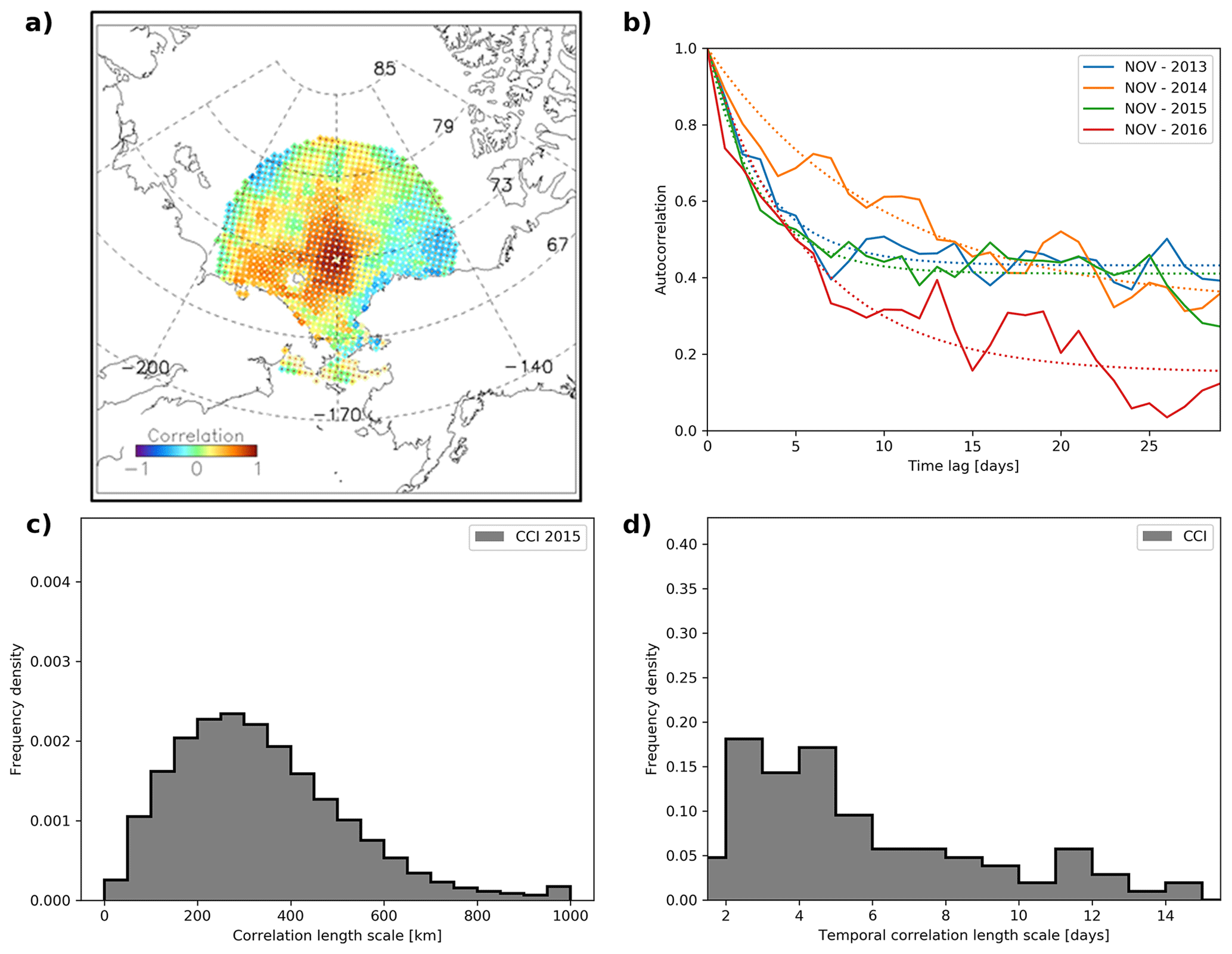
Figure 1Spatial (a, c) and temporal (b, d) correlation characteristics. (a) An example of the correlation with a selected location near Wrangel Island on 26 January 2010. (c) The frequency distribution of the scale of spatial sea-ice concentration error correlation length for the Northern Hemisphere and the whole year of 2015. (b) Examples of the auto-correlation values (solid lines) for the Northern Hemisphere in September from 2013 to 2016 with a minimal RMSD fit (dotted lines). (d) The frequency distribution of the temporal correlation length scale for the years 2013 to 2016 . Panel (a) is taken from Kern (2021).
Kern (2021) finds that the SIC error correlation length (used here) is generally larger than the total error correlation length (about 200 to 700 km compared to mostly below 200 km). Kern further identifies significant temporal and regional variability in the derived correlation length scale. Figure 1c shows that for 2015, the spatial error correlation length, as provided by Kern (2022), peaks at around 300 km. The generated samples will be designed to echo this distribution and, hence, have a variability similar to that of the correlation length scale in Kern (2022). Due to a lack of other information, we assume that this error correlation length can be applied to all locations, independent of the local SIC value.
2.1.2 Temporal correlation
In contrast to the spatial correlation length scales, we estimate the temporal error correlation length (i.e. the duration) ourselves but largely follow the processing of the spatial SIC error length in Kern (2021). Using the untruncated CCI SIC fields, we check each month for locations where the daily SIC never falls below 90 % SIC. Based on all these locations, we derive a monthly autocorrelation time series and find the minimum RMSD fit of an exponentially decaying function, ct(Δt) (Eq. 1, Fig. 1b). The e-folding value, ℓt, of this fit is used as a measure for the temporal error correlation length. The seasonal cycle and potential trends are not removed from the SIC data set for this processing because they are expected to have negligible impact on timescales of several days to weeks. However, we do allow ct to converge to a floor-level cf different from zero:
where Δt is the time lag and ℓt is the temporal error correlation length. The addition of a floor-level correlation results in much better fits of ct to the autocorrelation data (Fig. 1b), which improve the representation of the initial drop in autocorrelation of interest here.
2.2 Monte Carlo modelling
We use the previously identified spatial and temporal error correlations to create a Monte Carlo ensemble in order to propagate the CCI SIC uncertainty estimates to the SIA and SIE estimates. The spread within the SIC ensemble represents its correlated uncertainties. Therefore, the ensemble spread in the resulting SIA or SIE estimates provides an estimate of the propagated uncertainty.
The generation of ensemble members with correlated random errors consists of the following four steps. (1) Independent white noise with zero mean and a standard deviation of 1 is generated in the whole domain by a numerical random generator. The noise is generated for the whole time period and hemisphere at once to avoid discontinuities in the final error fields. (2) A three-dimensional Gaussian low-pass filter with sigma values of 5 d in the time dimension and 288 km in the two space dimensions (compare Fig. 1c and d) is applied to the independent noise to remove higher-frequency components. These nominal values are not matched exactly in the generated ensemble; the quality of the statistical model will be evaluated in the following section. Two alternative types of filters have been applied for comparison, which have limited impact on the results (see the Appendix). (3) The amplitude of the filtered noise field is normalized to have a standard deviation of 1. (4) The noise field is multiplied with the total_standard_error variable of the CCI SIC product. All noise realizations are added individually to daily fields of the SIC product from which the high-frequency variations have been filtered. The CCI SIC product contains errors itself; the objective here is to replace these errors by statistically generated ones. Therefore we remove high-frequency SIC variations using the same Gaussian filter on the SIC data, as is used to create errors fields. Without this step, we would add the generated error fields to an SIC field that already contains the same type of error so that the resulting fields would, by default, show stronger spatio-temporal variability.
2.3 Quality of generated noise
To examine the quality of the generated SIC field, we need to examine two questions describing the two basic quality measures mentioned before. (1) How well is the local spread within the ensemble reflecting the uncertainty estimates of the CCI SIC product? (2) How well does the generated ensemble reproduce the spatial and temporal error correlation characteristics of the original product? If both criteria are met, then we have shown that our synthetic errors are a good approximation for the inherent product errors.
2.3.1 Local uncertainties
To examine whether the first quality measure is met, we compare the spread in the generated ensemble with the uncertainty estimate by the data providers (Fig. 2). We find that, indeed, the ensemble spread is very similar to the total_standard_error variable, which is the combination of the algorithmic uncertainty and the smearing uncertainty, representing 1 standard deviation in percentage points of the SIC. It is outside the scope of this work to derive individual error characteristics for those contributing uncertainties. Note that we do not assess the quality of the local CCI SIC uncertainty estimate here but instead focus on creating a statistical representation of this product.
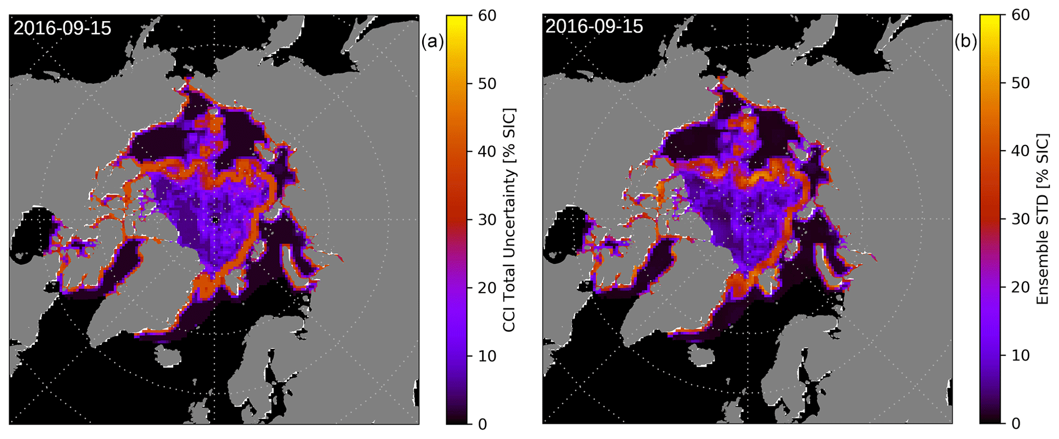
Figure 2Example of (a) uncertainty estimates as provided by the CCI SIC product total_standard_error variable and (b) the standard deviation of 100 members of the statistically generated ensemble using the Gaussian filtering approach.
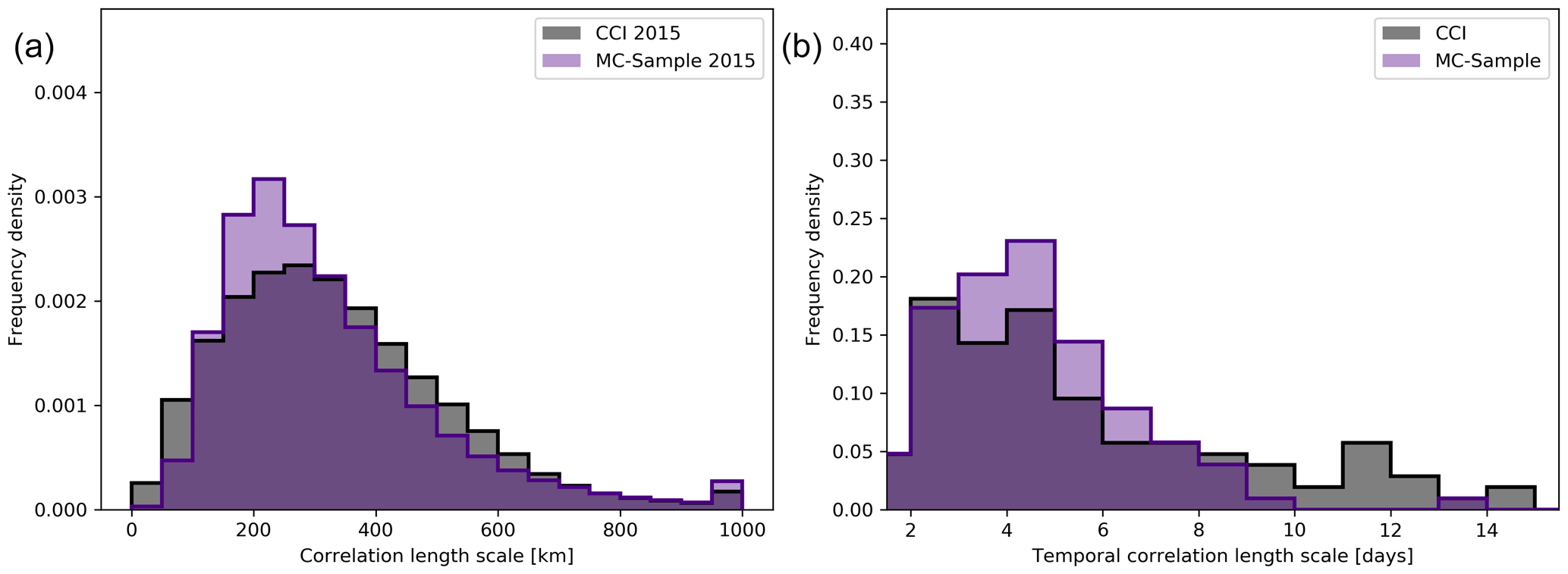
Figure 3Comparison of the error correlation distributions of the CCI SIC product with the statistically generated ensemble. The shown spatial distributions (a) for 2015 have a mean of 333 km (CCI) and 322 km (sample) and a median of 305 km (CCI) and 280 km (sample). The shown temporal error distributions (b) have a mean of 5.8 d (CCI) and 4.5 d (sample) as well as a median of 4.7 d (CCI) and 4.2 d (sample).
2.3.2 Error characteristics
The spatial and temporal error characteristics of the statistically generated ensemble members are similar to the ones of the original CCI SIC product (Fig. 3). For Fig. 3, we use the same approach to derive spatial and temporal error correlation lengths, as described in Sect. 2.1, on one noise realization to be compared with the CCI SIC characteristics. It can be seen that not only do the average correlation length scales agree between the CCI SIC and statistically generated ensemble members but also the width of the distributions is consistent.
In summary, we have generated a statistical ensemble of SIC time–space fields, which are centred around the CCI SIC product while the added noise is in excellent agreement with the local CCI SIC uncertainty estimates and the estimated temporal and spatial error correlations. In the following, we can therefore use the generated ensemble to quantify uncertainties in the SIA and SIE.
In order to derive SIA and SIE uncertainties, we repeat the calculation of daily SIA and SIE values for each ensemble member individually (Fig. 4a, b). Note that the temporal correlation in the SIC errors results in increased smoothness over time in the SIA and SIE variability in ensemble members compared to temporally independent noise (Fig. 4a, b; compare Fig. A1). The errors in SIA and SIE can neither be well represented by a constant bias nor by temporally independent noise, which highlights the value of our approach to statistically model the underlying SIC error. This can also be seen from the SIA and SIE anomalies (Fig. 4c, d), the spread of which also gives a first impression of the ensemble uncertainty.
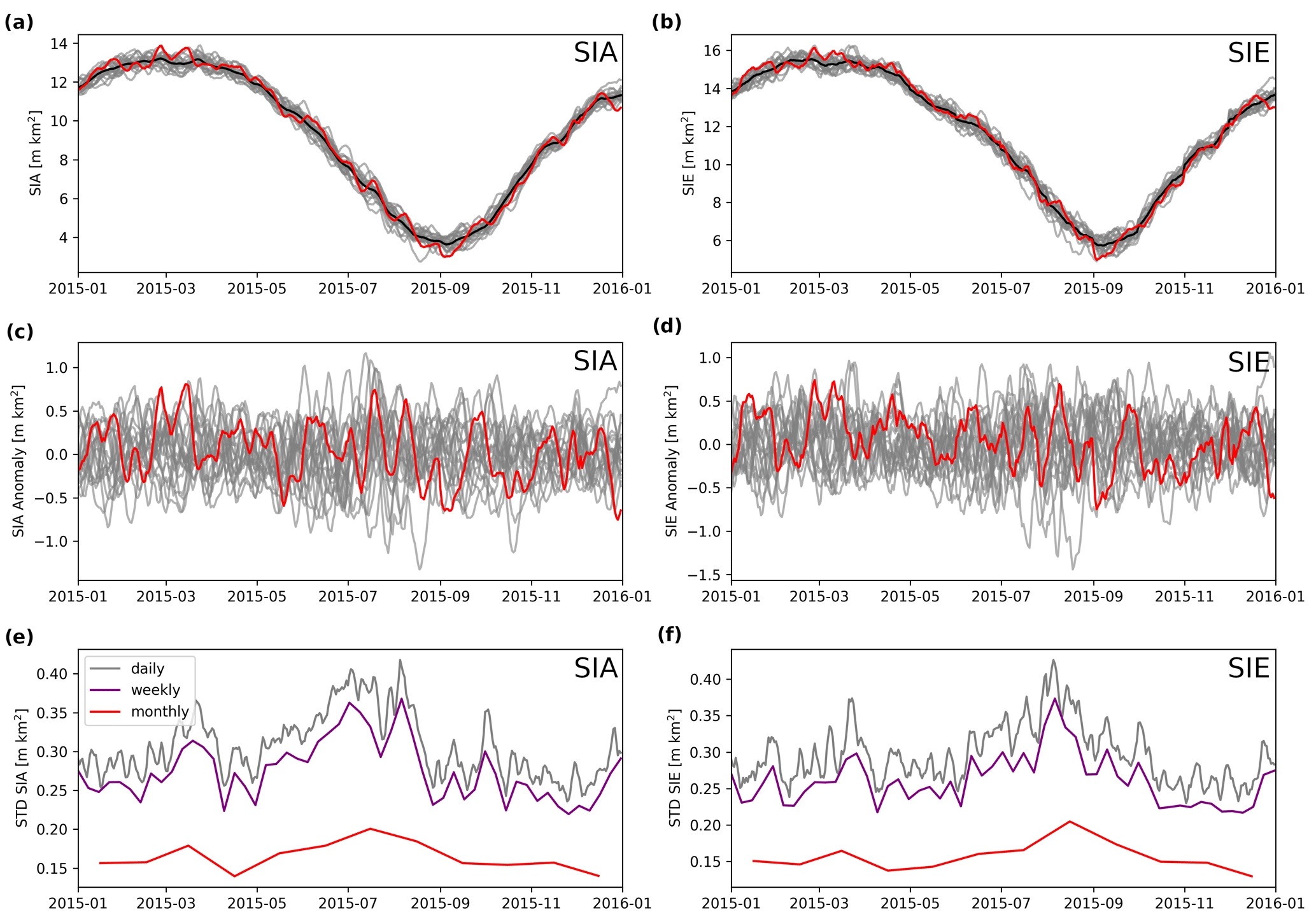
Figure 4Daily Arctic SIA (a, c, e) and SIE (b, d, f) ensemble for the year 2015 in grey and red with the ensemble mean shown in black. For illustration, only 20 out of 100 ensemble members are shown, one of which is highlighted in red to illustrate the temporal correlation of the time series. The SIA and SIE time series themselves are shown at the top; the anomalies with subtracted ensemble mean are shown in the middle; and the ensemble standard deviation of daily (grey), weekly (purple), and monthly (red) averages is shown in the bottom panels.
In a next step, we derive the weekly mean and monthly mean SIA and SIE estimates from the daily time series and afterwards calculate the corresponding ensemble SD (Fig. 4e, f). As an example, we find that the mean SIA uncertainty in 2015 is 306 000 km2 for daily estimates, 275 000 km2 for weekly estimates, and 164 000 km2 for monthly estimates. The SIE uncertainty in 2015 is slightly smaller with 296 000 km2 for daily estimates, 261 000 km2 for weekly estimates, and 156 000 km2 for monthly estimates.
This example shows that weekly averages have nearly the same uncertainty as daily estimates, which is due to the typical temporal error correlation of 5 d. In general, the uncertainty of daily SIA and SIE values strongly depends on the spatial error correlation, while the amount of uncertainty reduction by temporal averages is determined by the temporal correlation (see the Appendix, Fig. A1). The reduction in errors by weekly averages is small because errors do not cancel efficiently due to the temporal error correlation. For monthly estimates, in contrast, the uncertainty is reduced by a factor of about 2. Figure 4e and f indicate a small increase in SIA and SIE uncertainties in summer (JJA) compared to the rest of the year.
We address the sensitivity of our uncertainty estimates on the SIC error correlation length scales by repeating the ensemble generation for realistic lower-end and upper-end correlation length scales. The difference in daily uncertainty between these two setups is about 80 000 km2 for both SIA and SIE (Fig. A2 and Table A1).
Of particular interest both scientifically and in the public discussion is the trend in September SIA and SIE because September is the month that typically contains the yearly sea-ice minimum and is one of the months with the fastest observed decline in sea ice (Stroeve and Notz, 2018). We derive the linear trends of the ensemble members by a minimum RMSD fit to the September daily SIA estimates from 2002 to 2017 and analyse their statistical distribution (Fig. 5). Figure 5a shows that the ensemble spread in September SIA is notably different from year to year and gives a first indication for the spread in the linear trend. The distribution of the SIA ensemble trend for this period has a mean of 105 000 km2 a−1 with 1 standard deviation of about 9000 km2 a−1 (Fig. 5b). The standard error in the trend, estimated directly from the CCI SIC data, is nearly 6000 km2 a−1 and thus is similar to, yet slightly smaller than, our uncertainty estimate.
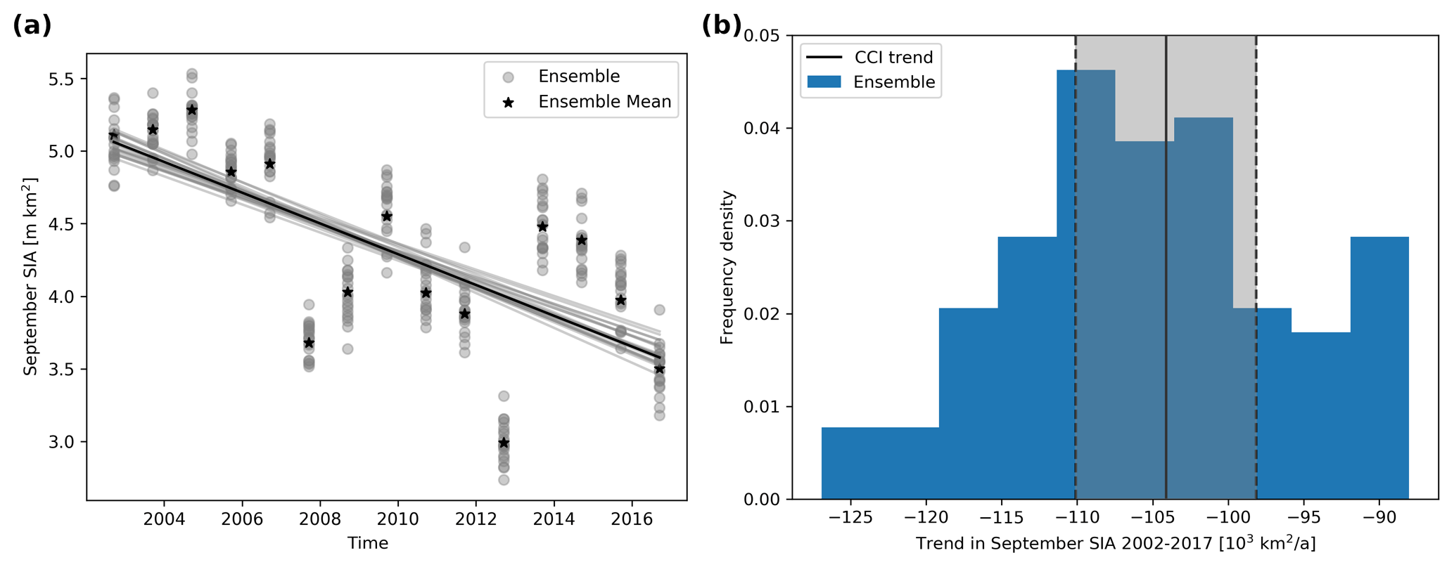
Figure 5(a) September SIA estimates from 2002 to 2017 for the first 20 ensemble members (grey) and the ensemble mean (black) with linear regression lines in corresponding colours. Note that September mean values are displayed to show the spread in the ensemble, while daily values are used for the regression. (b) Ensemble distribution of September SIA trends (blue) with the trend from the linear regression based directly on the CCI product, for comparison (black line), and 1 standard error in the trend (grey shading).
The uncertainties studied here can be understood as an improved representation of the total_standard_error variable provided with the ESA CCI sea-ice concentration product. We fully rely on the experience and extensive validation efforts of the data providers to quantify the local uncertainties (Kern and Timms, 2018). As mentioned in the Introduction, these uncertainty estimates summarize the impact of several sources of uncertainty. However, biases are not represented in these estimates; for example, those from the applied land mask, which would require a separate statistical treatment, are not represented.
The assumption of homogeneous and purely radial error correlations is of course a simplification: some sources of errors are expected to play a stronger role in specific conditions. This includes the land spill over, which originates from a strong contrast between microwave signatures from the land and the ocean, while the signatures of the land and sea ice are very similar. The passive microwave sensors permit a blurring of this sharp contrast, leading to a contamination of measurements near the coast with land signatures (Parkinson, 1987; Cavalieri et al., 1999), which can confuse the SIC retrievals. This leads to a potential SIC overestimation, in particular for low ice conditions near the coast where the contrast between ocean and land emissivities is largest. Filters to reduce the land spill-over effect exist and are also used in the CCI SIC product (Lavergne et al., 2019). Nevertheless, this effect is creating increased uncertainty in some cases and is likely to create correlated errors along the coast that lose correlation much quicker in an offshore direction.
Additional error sources with likely non-circular error correlations are tie-point errors. Errors in tie points are expected to create errors at all locations with conditions similar to the tie-point conditions. Therefore, error correlations are expected to be higher between locations with high sea-ice concentrations and between locations with low sea-ice concentrations. In other words, since the ocean and sea-ice tie points are defined independently of each other, one would expect the errors in an ocean measurement to be less correlated with errors in sea-ice measurements, everything else being equal.
Despite these caveats, we use a circular correlation pattern in this study, based purely on the distance between two locations. The existence of a non-circular correlation pattern is further supported, for example, by Fig. 5 in Kern (2021). However, taking these into account requires additional research to quantify the cause, abundance, and impact of those non-circular components. In general, an increase in error correlations at locations with high uncertainties, such as the coast and marginal ice zone, would correspond to larger uncertainties in the SIA and SIE.
Another assumption we rely on is that the error characteristics derived from nearly 100 % SIC are applicable for all ice conditions. A similar analysis for intermediate SIC is not possible because variations in real SIC and SIC errors cannot be distinguished. For conditions close to 0 % SIC at locations close to the ice edge, the approach used here and in Kern (2021) could be applied in principle, but there is a larger chance of ice floes passing through the area, again making the distinction difficult between errors and real SIC variations. For high SIC areas, leads or other openings in the ice can have the same effect, and we have to be clear that the approach to derive correlation length scales by Kern (2021), which we adapted here, cannot distinguish between a real signal in SIC >90 % and errors in the product. That being said, leads typically close or freeze over within days. Leads covered with thin ice can cause passive microwave products to show reduced SIC values, which we consider an error in the SIC estimate. Therefore, we want refrozen leads to be represented by the error ensemble. For a better understanding of error correlations, one would need a large set of high-quality reference data to be analysed for passive microwave SIC error characteristics, which currently do not exist.
We compare two trend uncertainty estimates of different natures: the traditional standard error in the trend, which is often provided with linear regressions, is based exclusively on the SIA values and is driven by the length of the time series and measurement-to-measurement variability. Our estimate is representing the measurement uncertainty, based on the propagation of the total_standard_error variable and is therefore not representing the influence of inter-annual variability. We realize that it can be confusing to use the same notation for different kinds of trend uncertainties and propose the use of the “measurement trend uncertainty” for the type of uncertainty produced here and the “standard error in the trend” or, more generally, the “trend fitting uncertainty” for the type of uncertainties based exclusively on the SIA values. Our measurement trend uncertainty here is less sensitive to the decision to fit the trend to daily or monthly mean SIA values (9151 vs. 9042 km2 a−1), while the standard errors in the trend (just as the p values, indicating the significance of trends) are very sensitive (5980 vs. 29 502 km2 a−1). This could be an effect of the inherent assumption of independence of uncertainties in the computation of the latter two, traditional quantities.
Comiso et al. (2017) compare four different SIC products and find the decline in the annual minimum SIA to be 79 300 km2 a−1 on average for the period from 1979 to 2015. This is smaller than the decline of about 105 000 km2 a−1 found here for the period from 2002 to 2017 (Fig. 5b). Since the decline in SIA is accelerating (e.g. Comiso et al., 2017), the differences can be easily explained by the different time periods used. The range between the products with the smallest (69 100 km2 a−1, NASA Team 1) and largest decline (85 800 km2 a−1, HadISST.2) in minimum SIA in Comiso et al. (2017) is 16 700 km2 a−1, or about 20 % of the average estimate. This range of inter-product uncertainty in the SIA trend is fully consistent with our single product ensemble uncertainty estimate where a single SD of the trend (9000 km2 a−1) corresponds to about 8.5 % of the average.
For a specific SIC data set, the work presented here looks at the year 2015 for a continuous time series and data from 2002–2017 for the September trend analysis (CCI SIC at 50 km resolution). It demonstrates how error estimates can be supplied for SIE and SIA estimates and for their trends. In a next step, our method can readily be implemented for sea-ice indicators on a daily basis by operational services such as the EUMETSAT OSI SAF. The implementation of our method by data providers could allow them to provide error estimates not only to daily and monthly mean SIE and SIA time series but also to set confidence intervals for other widely used metrics. Such metrics include the trends in monthly SIE and SIA (typically September and March) as well as rank values such as record low/high and earliest/latest sea-ice extremes. Such an implementation could, thus, increase the maturity of these key climate indicators. We further hope that this work will inspire the development of more sophisticated SIC error correlation estimates to refine SIA and SIE uncertainty estimates and improve the SIC ensemble from different SIC algorithms and new applications. If regional error characteristics are sufficiently well represented, then the SIC ensemble could be used directly in regional coupled models to investigate the impact of correlated SIC uncertainties in oceanic and atmospheric surface fluxes.
An analysis of errors in the CCI passive microwave SIC product indicates typical error correlations of around 300 km in space (based on the findings of Kern, 2021) and about 5 d in time. We derive a SIC error ensemble by statistical modelling and show that this ensemble is able to represent the local SIC uncertainty estimates as provided by the CCI SIC product and the analysed error correlations. These correlations are shown to have a strong impact on the error propagation from local SIC to aggregated SIA and SIE. The SIA uncertainty in 2015 is 306 000 km2 for daily estimates, 275 000 km2 weekly estimates, and 164 000 km2 for monthly estimates. The SIE uncertainty in 2015 is slightly smaller with 296 000 km2 for daily estimates, 261 000 km2 weekly estimates, and 156 000 km2 for monthly estimates. These daily uncertainties correspond to more than 5 % of the total SIA and SIE values around the yearly minimum. The uncertainties in weekly SIA and SIE averages are very similar to those of daily estimates due to the temporal error correlation. Quantitatively, these uncertainties are about half as large as the spread in SIA and SIE estimates from different products, which, however, differ not only by random errors as sampled here but also by conceptional factors such as different land masks (Kern et al., 2019) or the treatment of the pole hole in satellite data. These conceptional factors often result in biases. Uncertainties in SIE due to the algorithm parameter sensitivity of the order of 50 000 km2 a−1 as found by Meier and Stewart (2019) do not represent aspects like gridding and sensor noise. The uncertainties provided here originate from a single SIC product and encompass algorithmic and smearing uncertainties due to satellite footprint mismatches, which makes them a more appropriate estimate when, for example, comparing model and observational products on the same grid.
The Arctic September SIA trend for the period from 2002 to 2017 is estimated to be 105 000±9000 km2 a−1. This trend is an important indicator for the sensitivity of the Arctic ocean to climate change and a good example to illustrate the strength of our approach: biases (not represented here) are not an issue for trend analysis, but our improved representation of measurement uncertainties allows us to provide new insights into the trend uncertainty.
Using a simple (spatial- and temporal-)distance-based correlation model to propagate the uncertainties in the underlying SIC fields to uncertainties in the key climate indicators of SIA and SIE and their trends, we have been able to improve our understanding and the quantification of these uncertainties. We expect this quantification of observational uncertainties to be essential for our understanding of the ongoing Arctic climate change, both as a means in themselves and in providing a more robust basis for model evaluation studies.
The SIA and SIE uncertainty estimates are strongly dependent on the error correlation length scales. While we attempt to constrain the error correlation length as well as possible, there is some ambiguity in the best representation of these correlations. To investigate the impact of uncertainties in the error correlations, we test the sensitivities with regards to several aspects of the processing.
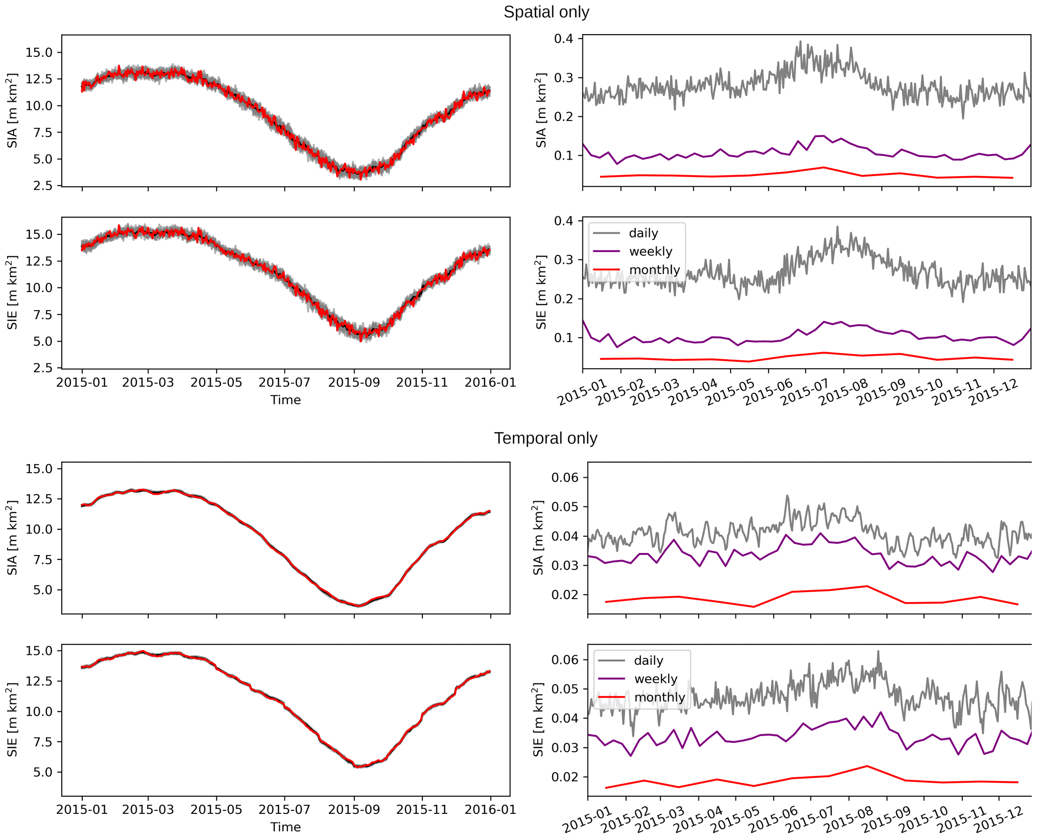
Figure A1Left: daily Arctic SIA and SIE ensemble of 20 SIC ensemble members with 1 member highlighted (red) and the mean (black). Right: standard deviations of SIA and SIE derived from an ensemble of 100 SIC ensemble members with only the (top) spatial error correlation and (bottom) temporal correlation.
A1 Sensitivity to individual correlations
First, we set the spatial (temporal) error correlation to zero and use our best estimate for the temporal (spatial) error correlation. In this way, we separate the impacts of the spatial and temporal correlations from each other (Fig. A1). We find that the spatial error correlation influences the magnitude of the SIA and SIE uncertainties, while the temporal correlation reduces the rate at which the uncertainties reduce with temporal averaging.
A2 Sensitivity to correlation length scales
Second, we define error correlations on the lower and upper end of consistency with observations. Based on Fig. 3, we choose ±50 km and ±1 d as a reasonable parameter range. We repeat the SIA and SIE uncertainty calculations for the combination of lower-end spatial and temporal error correlations (nominal 238 km and 4 d) as well as the combination of upper-end spatial and temporal error correlations (nominal 338 km and 6 d) in Fig. A2. These two setups can be understood as an envelope of SIA and SIE uncertainty estimates.
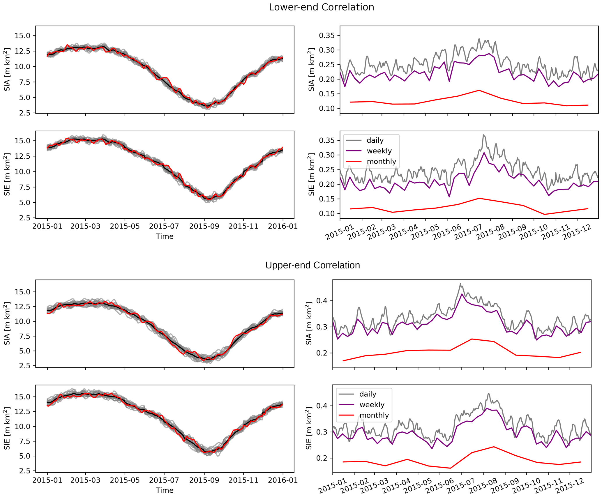
Figure A2Left: daily Arctic SIA and SIE ensemble of 20 SIC ensemble members with 1 member highlighted (red) and the mean (black). Right: standard deviations of SIA and SIE derived from an ensemble of 100 SIC ensemble members with (top) lower-end and (bottom) upper-end spatial and temporal error correlations.
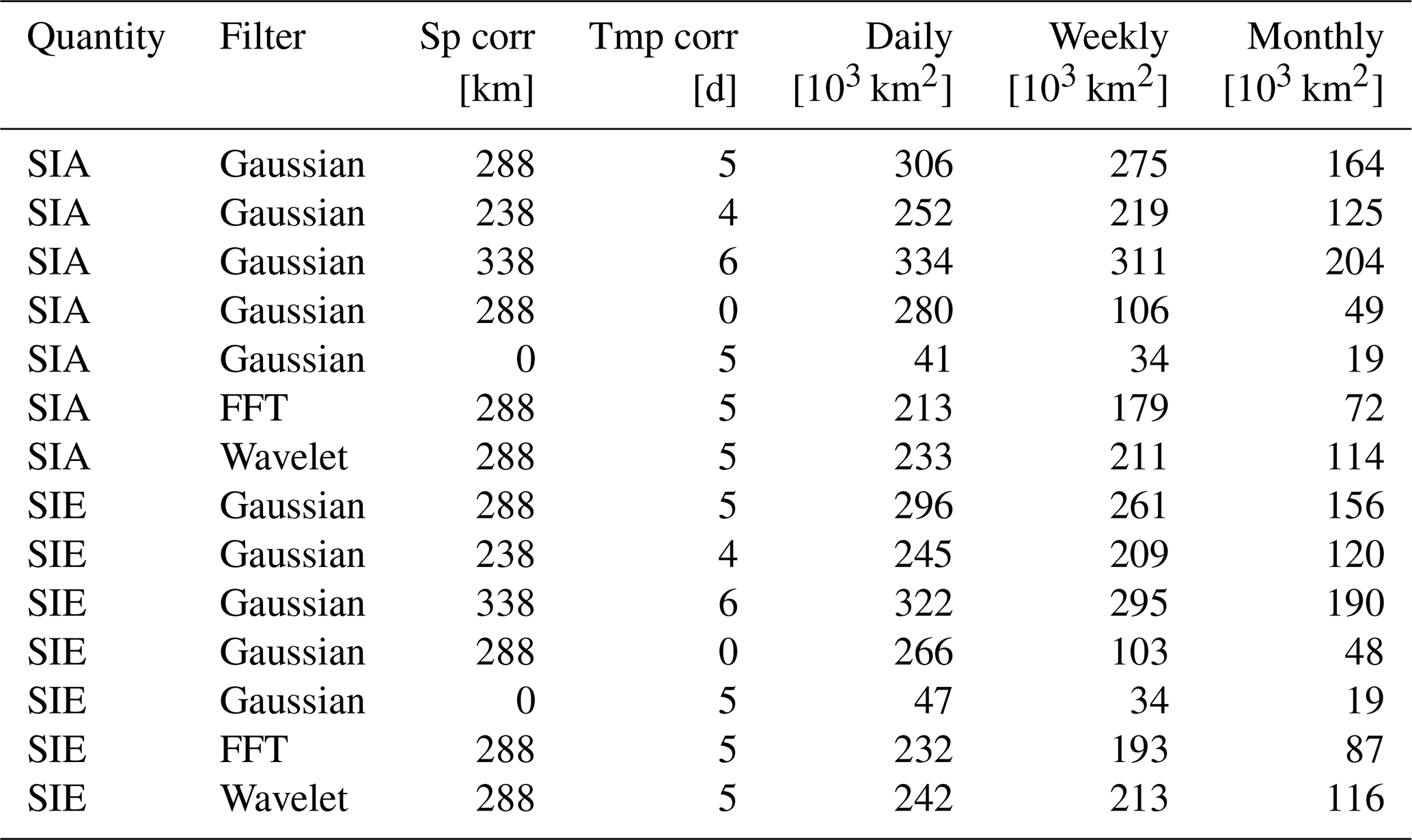
Table A1Uncertainty estimates (1 SD) of 100 ensemble members for the year 2015 based on different processing types. The spatial (Sp) and temporal (Tmp) error correlations are nominal values and do not necessarily correspond to the averaged analysed error correlations (see text).
A3 Sensitivity to the filter type
To assess the sensitivity to the filter type, we use two alternative filters to create the noise ensemble: a fast Fourier transform (FFT) and a wavelet filter (Xu et al., 1994). The FFT filter transforms the independent noise field into a frequency representation in which we set all frequency contributions outside a given range to zero. The inverse transformation creates the required noise in the space–time domain. The FFT is a global transformation, meaning that oscillating components in the whole noise field are preserved if they have a frequency which is not filtered out. This is important because it means that FFT bandpass filters have the tendency to create negative correlations at specific distances in addition to the desired positive correlation at small distances. Such anticorrelation is not expected to be found in SIC errors.
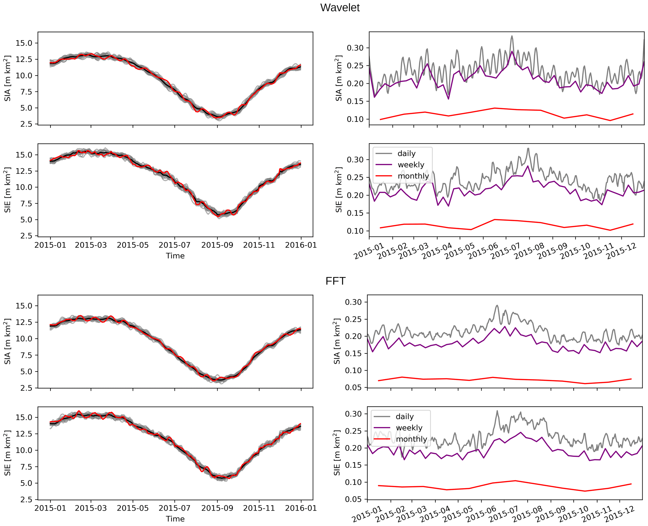
Figure A3Left: daily Arctic SIA and SIE ensemble of 20 SIC ensemble members with 1 member highlighted (red) and the mean (black). Right: standard deviations of SIA and SIE derived from an ensemble of 100 SIC ensemble members based (top) on a wavelet filter and (bottom) on a fast Fourier transform filter.
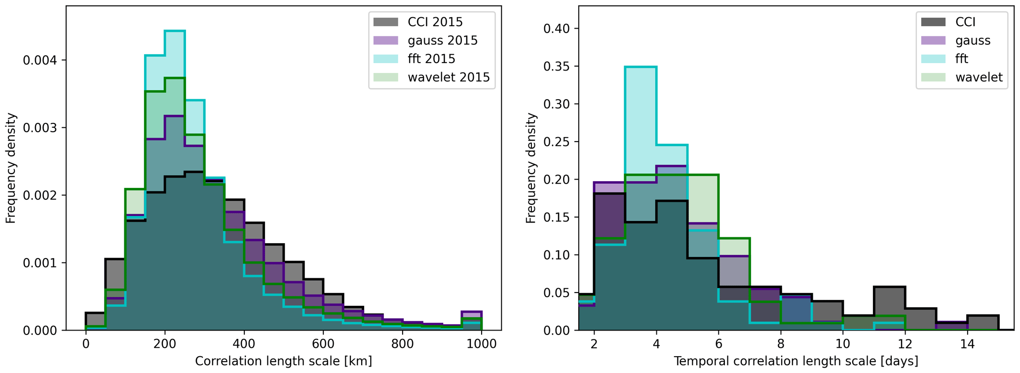
Figure A4The same as Fig. 3 but including noise characteristics from the wavelet filter and fast Fourier transform filter.
A wavelet transformation is a multi-resolution decomposition of an n-dimensional image. The basis functions (wavelets) are, in contrast to the FFT, diminishing with distance to their centre and are therefore supported only on local subsections of the image. Wavelet transforms are able to reveal the frequency content of the signal around a specific location, which makes them attractive to identify edges in noisy images (e.g. Xu et al., 1994). Differently sized wavelets, representing different frequencies, are used as a basis function for a wavelet decomposition, providing coefficients that illustrate at which location which frequency is found in the signal. Wavelet recompositions have been used to create geophysical noise in applications similar to ours (Castleman et al., 2022).
The filtering steps are the same for FFT and wavelet filters: first, the three-dimensional white noise field is decomposed into its frequency components. Then, frequency components/wavelet coefficients outside of a manually defined window are set to zero, followed by a reverse transformation/recomposition into the original space–time domain. For the FFT bandpass filter, the range is set from 238 to 338 km and from 4 to 6 d. The wavelet filter decomposes the noise field into four levels using a discrete wavelet transform with Daubechies-12 wavelets (function wavedecn() of the Python module pywt) and removes the contributions from the two smallest levels before recomposition. We have set these variables to reproduce spatial and temporal error correlation length scales as closely as possible (Fig. A4) in order to focus on the sensitivity of the functional form of the error correlations itself. Figure A3 and Table A1 show that the sensitivity of the SIA and SIE uncertainties to the used filter type is up to 93 000 km2. That being said, the FFT filter noise used here has slightly shorter spatial correlations (Fig. A4). As we have seen in Fig. A1, this leads to a smaller total SIA and SIE uncertainty, which is also what we see when comparing Fig. A3 with Fig. 4. Therefore, the quoted filter type sensitivity is likely to be overestimated and, in fact, smaller than the sensitivity to the correlation length scales.
The original SIC data are available from the ESA CCI website and the CEDA Archive (https://doi.org/10.5285/5f75fcb0c58740d99b07953797bc041e; Pedersen et al., 2017). The code to create ensemble members based on these data is available at https://doi.org/10.5281/zenodo.7244321 (Wernecke, 2022).
AW designed the study, conducted the analysis, and wrote the first version of the manuscript. DN advised on the study design, SK helped, in particular, with the use of spatial correlation estimates and processed data specifically for this study. TL advised on the CCI uncertainty estimates. All authors engaged in discussions, which where absolutely essential for this project, and in manuscript revisions.
The contact author has declared that none of the authors has any competing interests.
Publisher's note: Copernicus Publications remains neutral with regard to jurisdictional claims made in the text, published maps, institutional affiliations, or any other geographical representation in this paper. While Copernicus Publications makes every effort to include appropriate place names, the final responsibility lies with the authors.
The authors are thankful to the two anonymous reviewers.
This work was supported by the ESA Climate Change Initiative CMUG project. Andreas Wernecke, Dirk Notz, and Thomas Lavergne also acknowledge the support given by the ESA Climate Change Initiative Sea Ice project (contract no. 4000126449/19/I-NB), and Dirk Notz acknowledges the funding by the Deutsche Forschungsgemeinschaft (DFG) under Germany's Excellence Strategy – EXC 2037 “CLICCS – Climate, Climatic Change, and Society” (project no. 390683824).
The article processing charges for this open-access publication were covered by the Max Planck Society.
This paper was edited by John Yackel and reviewed by two anonymous referees.
Alekseeva, T., Tikhonov, V., Frolov, S., Repina, I., Raev, M., Sokolova, J., Sharkov, E., Afanasieva, E., and Serovetnikov, S.: Comparison of Arctic Sea Ice concentrations from the NASA team, ASI, and VASIA2 algorithms with summer and winter ship data, Remote Sens.-Basel, 11, 2481, https://doi.org/10.3390/rs11212481, 2019. a, b, c
Andersen, S., Tonboe, R., Kaleschke, L., Heygster, G., and Pedersen, L. T.: Intercomparison of passive microwave sea ice concentration retrievals over the high-concentration Arctic sea ice, J. Geophys. Res.-Oceans, 112, C8004, https://doi.org/10.1029/2006JC003543, 2007. a
Castleman, B. A., Schlegel, N.-J., Caron, L., Larour, E., and Khazendar, A.: Derivation of bedrock topography measurement requirements for the reduction of uncertainty in ice-sheet model projections of Thwaites Glacier, The Cryosphere, 16, 761–778, https://doi.org/10.5194/tc-16-761-2022, 2022. a
Cavalieri, D. J., Parkinson, C. L., Gloersen, P., Comiso, J. C., and Zwally, H. J.: Deriving long-term time series of sea ice cover from satellite passive-microwave multisensor data sets, J. Geophys. Res.-Oceans, 104, 15803–15814, https://doi.org/10.1029/1999JC900081, 1999. a
Comiso, J. C., Meier, W. N., and Gersten, R.: Variability and trends in the Arctic Sea ice cover: Results from different techniques, J. Geophys. Res.-Oceans, 122, 6883–6900, https://doi.org/10.1002/2017JC012768, 2017. a, b, c
Ding, Q., Schweiger, A., L’Heureux, M., Battisti, D. S., Po-Chedley, S., Johnson, N. C., Blanchard-Wrigglesworth, E., Harnos, K., Zhang, Q., Eastman, R., and Steig, E. J.: Influence of high-latitude atmospheric circulation changes on summertime Arctic sea ice, Nat. Clim. Change, 7, 289–295, https://doi.org/10.1038/nclimate3241, 2017. a, b
Ding, Q., Schweiger, A., L’Heureux, M., Steig, E. J., Battisti, D. S., Johnson, N. C., Blanchard-Wrigglesworth, E., Po-Chedley, S., Zhang, Q., Harnos, K., Bushuk, M., Markle, B., and Baxter, I.: Fingerprints of internal drivers of Arctic sea ice loss in observations and model simulations, Nat. Geosci., 12, 28–33, https://doi.org/10.1038/s41561-018-0256-8, 2019. a
Fox-Kemper, B., Hewitt, H. T., Xiao, C., Aoalgeirsdóttir, G., Drijfhout, S. S., Edwards, T. L., Golledge, N. R., Hemer, M., Kopp, R. E., Krinner, G., Mix, A., Notz, D., Nowicki, S., Nurhati, I. S., Ruiz, L., Sallée, J.-B., Slangen, A. B. A., and Yu, Y.: Ocean, Cryosphere and Sea Level Change, Chap. 9, Cambridge University Press, Cambridge, United Kingdom and New York, NY, USA, https://doi.org/10.1017/9781009157896.011, 2021. a, b
Gulev, S. K., Thorne, P. W., Ahn, J., Dentener, F. J., Domingues, C. M., Gerland, S., Gong, D., Kaufman, D. S., Nnamchi, H. C., Quaas, J., Rivera, J. A., Sathyendranath, S., Smith, S. L., Trewin, B., von Schuckmann, K., ose, R. S., Allan, R., Collins, B., Turner, A., and Hawkins, E.: Changing state of the climate system, Chap. 2, Cambridge University Press, Cambridge, United Kingdom and New York, NY, USA, https://doi.org/10.1017/9781009157896.004, 2021. a
Ivanova, N., Johannessen, O. M., Pedersen, L. T., and Tonboe, R. T.: Retrieval of Arctic sea ice parameters by satellite passive microwave sensors: A comparison of eleven sea ice concentration algorithms, IEEE T. Geosci. Remote, 52, 7233–7246, https://doi.org/10.1109/TGRS.2014.2310136, 2014. a
Ivanova, N., Pedersen, L. T., Tonboe, R. T., Kern, S., Heygster, G., Lavergne, T., Sørensen, A., Saldo, R., Dybkjær, G., Brucker, L., and Shokr, M.: Inter-comparison and evaluation of sea ice algorithms: towards further identification of challenges and optimal approach using passive microwave observations, The Cryosphere, 9, 1797–1817, https://doi.org/10.5194/tc-9-1797-2015, 2015. a
Kay, J. E., Holland, M. M., and Jahn, A.: Inter-annual to multi-decadal Arctic sea ice extent trends in a warming world, Geophys. Res. Lett., 38, L15708, https://doi.org/10.1029/2011GL048008, 2011. a, b, c
Kern, S.: Spatial Correlation Length Scales of Sea-Ice Concentration Errors for High-Concentration Pack Ice, Remote Sens.-Basel, 13, 4421, https://doi.org/10.3390/rs13214421, 2021. a, b, c, d, e, f, g, h, i, j, k
Kern, S.: Spatial correlation length scales of sea-ice concentration errors of high-concentration pack ice for ESA-CCI-SICCI2-50km (Version 2022_fv0.01), Research Data Repository of Universität Hamburg [data set], https://doi.org/10.25592/uhhfdm.10413, 2022. a, b, c
Kern, S. and Timms, G.: Sea Ice Climate Change Initiative: Phase 2 Product Validation & Intercomparison Report (PVIR) version 1.1, Tech. rep., ESA, https://climate.esa.int/media/documents/Sea_Ice_Concentration_Product_Validation_and_Intercomparison_Report_1.1.pdf (last access: 16 May 2024), 2018. a
Kern, S., Lavergne, T., Notz, D., Pedersen, L. T., Tonboe, R. T., Saldo, R., and Sørensen, A. M.: Satellite passive microwave sea-ice concentration data set intercomparison: closed ice and ship-based observations, The Cryosphere, 13, 3261–3307, https://doi.org/10.5194/tc-13-3261-2019, 2019. a, b, c, d
Kern, S., Lavergne, T., Notz, D., Pedersen, L. T., and Tonboe, R.: Satellite passive microwave sea-ice concentration data set inter-comparison for Arctic summer conditions, The Cryosphere, 14, 2469–2493, https://doi.org/10.5194/tc-14-2469-2020, 2020. a, b
Kern, S., Lavergne, T., Pedersen, L. T., Tonboe, R. T., Bell, L., Meyer, M., and Zeigermann, L.: Satellite passive microwave sea-ice concentration data set intercomparison using Landsat data, The Cryosphere, 16, 349–378, https://doi.org/10.5194/tc-16-349-2022, 2022. a
Lavergne, T., Sørensen, A. M., Kern, S., Tonboe, R., Notz, D., Aaboe, S., Bell, L., Dybkjær, G., Eastwood, S., Gabarro, C., Heygster, G., Killie, M. A., Brandt Kreiner, M., Lavelle, J., Saldo, R., Sandven, S., and Pedersen, L. T.: Version 2 of the EUMETSAT OSI SAF and ESA CCI sea-ice concentration climate data records, The Cryosphere, 13, 49–78, https://doi.org/10.5194/tc-13-49-2019, 2019. a, b, c
Meier, W. N.: Comparison of passive microwave ice concentration algorithm retrievals with AVHRR imagery in Arctic peripheral seas, IEEE T. Geosci. Remote, 43, 1324–1337, https://doi.org/10.1109/TGRS.2005.846151, 2005. a
Meier, W. N. and Stewart, J. S.: Assessing uncertainties in sea ice extent climate indicators, Environ. Res. Lett., 14, 035005, https://doi.org/10.1088/1748-9326/aaf52c, 2019. a, b, c
Mironov, D., Ritter, B., Schulz, J.-P., Buchhold, M., Lange, M., and MacHulskaya, E.: Parameterisation of sea and lake ice in numerical weather prediction models of the German Weather Service, Tellus A, 64, 17330, https://doi.org/10.3402/tellusa.v64i0.17330, 2012. a
Notz, D. and Marotzke, J.: Observations reveal external driver for Arctic sea-ice retreat, Geophys. Res. Lett., 39, L08502, https://doi.org/10.1029/2012GL051094, 2012. a, b, c
Notz, D. and SIMIP Community: Arctic sea ice in CMIP6, Geophys. Res. Lett., 47, e2019GL086749, https://doi.org/10.1029/2019GL086749, 2020. a, b
Parkinson, C. L.: Arctic sea ice, 1973-1976: Satellite passive-microwave observations, vol. 490, Scientific and Technical Information Branch, National Aeronautics and Space, 1987. a
Pedersen, L. T., Dybkjær, G., Eastwood, S., Heygster, G., Ivanova, N., Kern, S., Lavergne, T., Saldo, R., Sandven, S., Sørensen, A., and Tonboe, R.: ESA Sea Ice Climate Change Initiative (Sea_Ice_cci): Sea Ice Concentration Climate Data Record from the AMSRE and AMSR2 instruments at 50km grid spacing, version 2.1, Centre for Environmental Data Analysis [data set], https://doi.org/10.5285/5f75fcb0c58740d99b07953797bc041e, 2017. a, b
Roach, L. A., Dörr, J., Holmes, C. R., Massonnet, F., Blockley, E. W., Notz, D., Rackow, T., Raphael, M. N., O'Farrell, S. P., Bailey, D. A., and Bitz, C. M.: Antarctic sea ice area in CMIP6, Geophys. Res. Lett., 47, e2019GL086729, https://doi.org/10.1029/2019GL086729, 2020. a, b
Stroeve, J. and Notz, D.: Changing state of Arctic sea ice across all seasons, Environ. Res. Lett., 13, 103001, https://doi.org/10.1088/1748-9326/aade56, 2018. a, b
Stroeve, J., Holland, M. M., Meier, W., Scambos, T., and Serreze, M.: Arctic sea ice decline: Faster than forecast, Geophys. Res. Lett., 34, L09501, https://doi.org/10.1029/2007GL029703, 2007. a
Sun, Y., Ye, Y., Wang, S., Liu, C., Chen, Z., and Cheng, X.: Evaluation of the AMSR2 Ice Extent at the Arctic Sea Ice Edge using a SAR-based Ice Extent Product, IEEE T. Geosci. Remote, 61, 4205515, https://doi.org/10.1109/TGRS.2023.3281594, 2023. a, b
Tonboe, R. T., Eastwood, S., Lavergne, T., Sørensen, A. M., Rathmann, N., Dybkjær, G., Pedersen, L. T., Høyer, J. L., and Kern, S.: The EUMETSAT sea ice concentration climate data record, The Cryosphere, 10, 2275–2290, https://doi.org/10.5194/tc-10-2275-2016, 2016. a, b
Tonboe, R. T., Nandan, V., Mäkynen, M., Pedersen, L. T., Kern, S., Lavergne, T., Øelund, J., Dybkjær, G., Saldo, R., and Huntemann, M.: Simulated Geophysical Noise in Sea Ice Concentration Estimates of Open Water and Snow-Covered Sea Ice, IEEE J. Sel. Top. Appl. Earth Obs., 15, 1309–1326, https://doi.org/10.1109/JSTARS.2021.3134021, 2021. a
Wen, J., Wu, X., You, D., Ma, X., Ma, D., Wang, J., and Xiao, Q.: The main inherent uncertainty sources in trend estimation based on satellite remote sensing data, Theor. Appl. Climatol., 151, 915–934, https://doi.org/10.1007/s00704-022-04312-0, 2023. a
Wernecke, A.: Script to create MC ensemble to represent uncertainties in ESA CCI SIC dataset, Zenodo [code], https://doi.org/10.5281/zenodo.7244321, 2022. a
Xu, Y., Weaver, J. B., Healy, D. M., and Lu, J.: Wavelet transform domain filters: a spatially selective noise filtration technique, IEEE T. Image Process., 3, 747–758, https://doi.org/10.1109/83.336245, 1994. a, b