the Creative Commons Attribution 4.0 License.
the Creative Commons Attribution 4.0 License.
 | 17 May 2024
Geothermal heat source estimations through ice flow modelling at Mýrdalsjökull, Iceland
Eyjólfur Magnússon
Krista Hannesdóttir
Joaquín M. C. Belart
Finnur Pálsson
Geothermal heat sources beneath glaciers and ice caps influence local ice-dynamics and mass balance but also control ice surface depression evolution as well as subglacial water reservoir dynamics. Resulting jökulhlaups (i.e., glacier lake outburst floods) impose danger to people and infrastructure, especially in Iceland, where they are closely monitored. Due to hundreds of meters of ice, direct measurements of heat source strength and extent are not possible. We present an indirect measurement method which utilizes ice flow simulations and glacier surface data, such as surface mass balance and surface depression evolution. Heat source locations can be inferred accurately to simulation grid scales; heat source strength and spatial distributions are also well quantified. Our methods are applied to the Mýrdalsjökull ice cap in Iceland, where we are able to refine previous heat source estimates.
- Article
(8000 KB) - Full-text XML
- BibTeX
- EndNote


The role of subglacial geothermal heat in the mass balance and dynamics of glaciers and ice sheets has in recent years gained increased attention (e.g., Winsborrow et al., 2010; Smith-Johnsen et al., 2020a, b; Dziadek et al., 2021). In Iceland, basal melting due to geothermal and volcanic activity makes a significant contribution to glacier mass balance (Jóhannesson et al., 2020; Björnsson and Pálsson, 2008), particularly where the glaciers cover the volcanic zones of Iceland (Fig. 1). This applies to our study area, the Mýrdalsjökull ice cap at the southern coast of Iceland, covering the central volcano Katla (Larsen et al., 2013), where the estimated basal melting by geothermal activity is ∼0.15 , averaged over the entire ice cap (Jarosch et al., 2020; Jóhannesson et al., 2020).
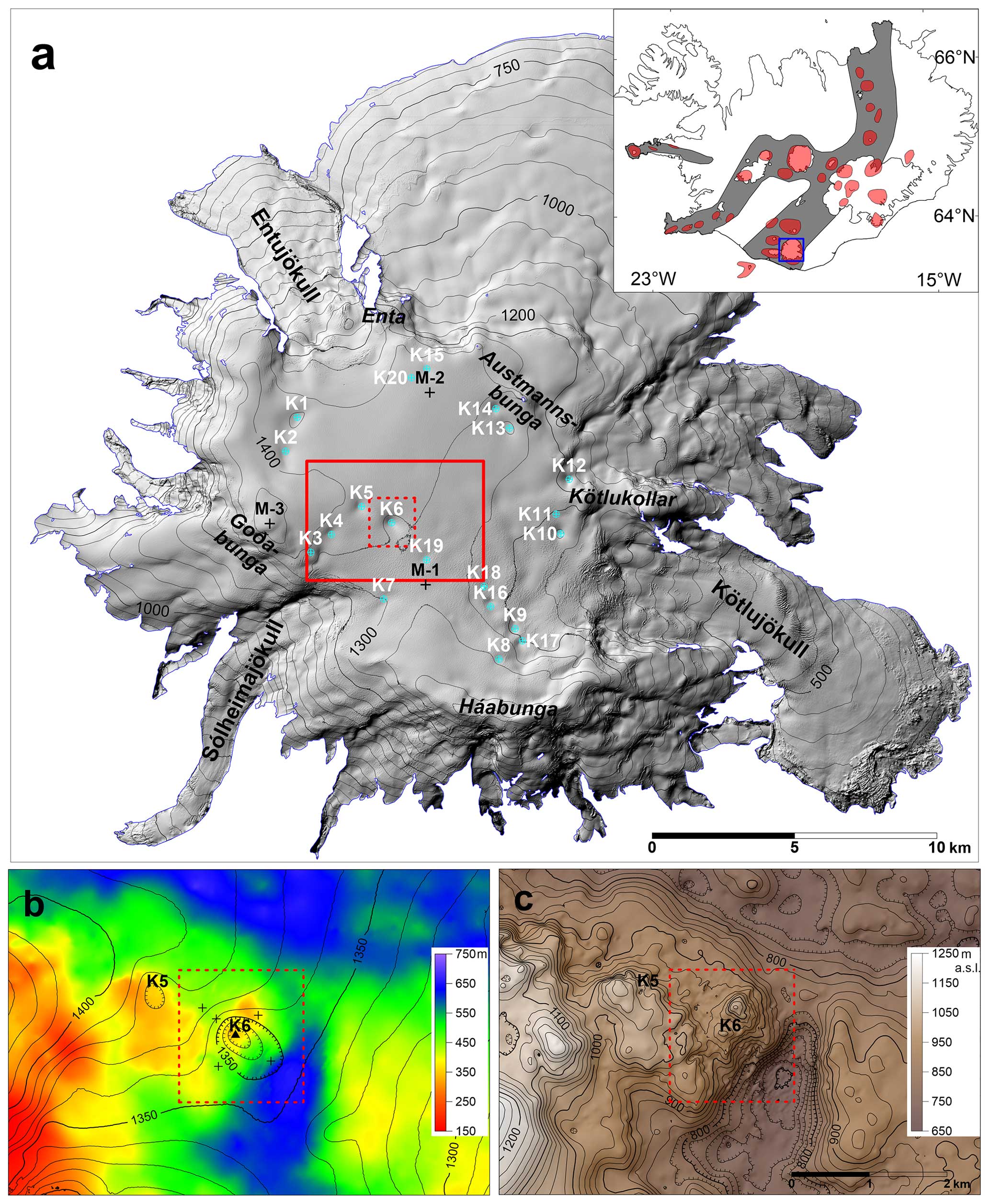
Figure 1(a) Mýrdalsjökull ice cap as a shaded relief image and a contour map (100 m elevation contour interval) using a surface DEM obtained in 2010 (Jóhannesson et al., 2013). The solid red line indicates the modelled area, and the dashed red line (also in panels b and c) indicates the focus area of this study. Names of outlet glaciers, glacier peaks and ice cauldrons formed by geothermal activity (white labels) are shown as well as mass balance survey locations (M-1, M-2 and M-3) in the accumulation area of Mýrdalsjökull. The inserted map indicates the geographic location of Mýrdalsjökull (blue square) along with the neo-volcanic zones (grey) of Iceland and active central volcanoes (red). (b) The glacier surface (contours with 10 m elevation interval) and ice thickness (image map) of the modelled area in 2016 (Magnússon et al., 2021). Locations of cauldrons K5 and K6 are shown. Crosses indicate locations of ablation survey sites in the summer of 2017; the triangle indicates a Global navigation satellite system (GNSS) station (and an ablation survey site) operated in the summers of 2016 and 2017. (c) The bedrock of the modelled area (Magnússon et al., 2021), shown as a contour map (20 m elevation interval). Hatched contours in panels (b) and (c) indicate closed depressions.
Geothermal as well as volcanic heat sources under glaciers influence local ice flow patterns and create distinct surface depressions (ice cauldrons), which are characteristic for sustained basal melt (e.g., Björnsson, 1988). Often, direct measurements of geothermal heat flux is impractical or even impossible due to the extensive ice thickness. Indirect estimations have been carried out using ice flow simulations (e.g., Jarosch and Gudmundsson, 2007). Over 20 ice cauldrons have been identified in the surface of Mýrdalsjökull, all of them located at or within the rim of the ice-covered caldera of Katla (Björnsson et al., 2000; Magnússon et al., 2021). The basal melt along with surface meltwater sometimes accumulates beneath the ice cauldrons, which can result in hazardous jökulhlaups (glacier lake outburst floods). Since the mid-20th century, three jökulhlaups (in 1955, 1999 and 2011), all with peak flow likely exceeding 1000 m3 s−1, have originated from underneath the ice cauldrons of Mýrdalsjökull, and they have destroyed roads, bridges and power lines (Þórarinsson and Rist, 1955; Sigurðsson et al., 2000; Guðmundsson and Högnadóttir, 2011). The risk of jökulhlaups has provoked regular monitoring of the ice cauldrons of Mýrdalsjökull (Guðmundsson et al., 2007; Magnússon et al., 2017) as well as detailed mapping of the bedrock topography beneath the ice cauldrons (Magnússon et al., 2021). These efforts have provided unique datasets which allow us to extend the two-dimensional simulations described in Jarosch and Gudmundsson (2007) to three dimensions in the attempt to resolve basal heat flux distributions. In this contribution, we present a novel, straightforward method to infer basal heat flux locations and distributions which utilizes three-dimensional ice flow simulations that account for basal melting. Input data to our method consist of ice surface topography, bedrock topography and specific glacier mass balance.
2.1 Data
Digital elevation models (DEMs) of the glacier surface and bedrock are used as inputs to our model. The surface DEM was derived from Pléiades optical high-resolution satellite images from 27 September 2016 (Magnússon et al., 2021), originally processed using the Ames Stereo Pipeline (Shean et al., 2016; Belart et al., 2020), with pixel size of 4×4 m and corrected for vertical bias using GNSS profiles obtained on 26 September 2016. For this study, the DEM was subsampled to 20×20 m pixels and further corrected by subtracting the measured new snow thickness of 1.15 m in K6 (K# refers to the various surface cauldrons; see Fig. 1 for their locations) on 26 September. The glacier surface input model therefore represents the glacier surface at the end of the ablation period, before the onset of the winter accumulation. The bedrock DEM has a pixel size of 20×20 m. It is based on radio echo sounding (RES) in 2016–2017 with the main area of interest beneath K6, deduced from traced bed reflections in 3D-migrated radar profiles surveyed with 20 m between profiles (Magnússon et al., 2021), resulting in a DEM based on more or less continuous measurements. The area outside K6 is derived from traced bed reflections in 2D-migrated RES profiles using Kriging interpolation. The density of the profiles is such that the distance between the nearest point of traced bed reflection is <100 m for the area of K5 but may be up to 200 m at some location outside the two cauldrons. Except for the area beneath K6, the bedrock DEM can therefore be subject to interpolation errors and errors caused by the limitation of the 2D migrated RES data (see Fig. 5 in Magnússon et al., 2021). For validation of modelling results (cf. Sect. 2.4), we use a DEM of the glacier surface from Pléiades images on 1 September 2017 which also has been processed using the Ames Stereo Pipeline (Shean et al., 2016; Belart et al., 2020). This DEM was co-registered to the 2016 DEM to ensure that the elevation difference pattern, caused by horizontal shift between the DEMs, was minimal. Furthermore, it was corrected for vertical bias using GNSS profiles obtained on 23–24 August 2017. No winter accumulation had started at that time, but the summer mass balance at survey sites in the accumulation area of Mýrdalsjökull (Fig. 1a) was measured during this field trip. From here onward, this glacier surface is referred to as H2017. To compensate for surface changes caused by surface mass balance, from autumn 2016 to autumn 2017, two different approaches are applied.
2.2 Numerical model
Simulating ice surface deformation driven by basal melting (i.e., negative basal mass balance) due to geothermal heat requires three interacting model components: ice dynamics, a suitable basal melting description and free surface motion. Ice dynamics are simulated using the well-established finite element model Elmer/Ice (Gagliardini et al., 2013), which solves the “full-Stokes” ice flow equations for standard, temperate ice (Glen's rate factor and Glen's nonlinearity n=3, values which were confirmed to be fitting the glacier motion, observed at GNSS stations and survey stakes, in Jarosch et al., 2020). Bounded by surface and bed topography (cf. Sect. 2.1), steady-state ice velocities (v) are computed for predefined basal melting configurations. These ice velocities are subsequently used to evolve the ice surface forward in time (cf. Eq. 3 below). We utilize a stress-free surface boundary condition in combination with no-flow () lateral boundary conditions for our model domain (cf. solid red box in Fig. 1). As we are interested in the local influence of basal melting on small-scale surface depression evolution, these lateral boundary conditions are legitimate for a sufficiently large model domain. The basal boundary is also defined as a no-flow boundary condition, except for regions where we prescribe a vertical ice outflow velocity () to represent basal melting (cf. Eq. 1 below) in our numerical model. Our computational grid follows the basal and surface topography on a 20 m resolution, with a Delaunay triangulated 2D mesh which is vertically extruded into 12 layers to create the computational domain. Basal melting, defined by a given heat flux (qh) distribution at the base of the glacier, is converted to a basal, vertical ice outflow velocity (vz,bh) distribution which is part of the Dirichlet velocity boundary condition for the ice flow model (e.g., Jarosch and Gudmundsson, 2007). Assuming instantaneous melting and drainage, vertical ice outflow velocities can be defined such that
Latent heat of fusion for ice is denoted as L and density of ice as ρ. Basal heat flux in Eq. (1) is given in W m−2; thus, a corresponding outflow velocity is computed for each square meter within a given heat flux distribution. Hence, the effect of spatial variations in heat flux on ice dynamics can be simulated.
Based on a computed ice velocity field, surface ice velocities can be extracted, and the vertical motion of ice surface elevations (s) is often computed according to
i.e., the kinematic boundary condition for shallow flows (e.g., Kundu et al., 2016), with being the surface mass balance rate of the glacier. Assumptions applied regarding are explained in Sect. 2.4. A detailed analysis on solving the free surface motion of glaciers utilizing Eq. (2) has been carried out by Wirbel and Jarosch (2020). In the work presented here, we do not rely on Eq. (2) and can treat the surface evolution of a glacier differently as we have dealt with surface mass balance in the input data processing (cf. Sect. 2.3), and we are not constrained by horizontally fixed grid points in our numerical methods. Applying a moving grid approach, we can evolve the three-dimensional surface point coordinate vector at each surface grid point i forward in time () by
utilizing the computed ice surface velocities vi,s.
To study the suitability of a given, prescribed basal heat flux distribution under our target glacier, we do the following:
-
compute the corresponding basal ice outflow distribution at the glacier bed with Eq. (1),
-
utilize the computed ice outflow velocities in combination with ice geometry to compute a three-dimensional ice velocity field with Elmer/Ice (cf. Fig. 2),
-
extract ice surface velocity components and move the ice surface geometry forward in time with Eq. (3) and a predefined time step (cf. Sect. 2.4),
-
compare the resulting ice surface geometry with reference data (cf. Sect. 2.1 and 2.4).
2.3 Simulation data processing
To focus our study on cauldron K6, we need to compensate for the effects of the much smaller heat source beneath K5. We do this by setting the outflow velocity at the bed to a fixed value of m yr−1 for a circular area with radius of 50 m beneath cauldron K5. This corresponds to a heat source with total power of 10 MW, but this rough estimate was based on a value from Jarosch et al. (2020) for the combined power of K5 and K6 in 2016–2017 (70±38 MW), considering that K5 is, by far, a shallower cauldron than K6 (Fig. 1b).
For K6, the heat flux distribution is assumed to follow a radially symmetric Gaussian distribution (cf. Fig. 2) such that the resulting vertical outflow velocity component (Eq. 1) is
Here, UZ0 is the peak outflow velocity, and σ is the standard deviation of the heat flux distribution. The solution of Eq. (4) is spatially limited inside a circle with radius R centered at coordinates (CX,CY). Outside that circle, solutions of Eq. (4) are set to zero.
Table 1Locations and geometry of the heat sources beneath K6 used in the presented simulations as well as results from comparison with validation data. Run numbers with Roman numerals indicate simulations that have been initially used to study the parameter space, whereas Arabic numerals are used for simulations that are discussed in detail. Run XI uses a constant vertical outflow velocity instead of a Gaussian distribution.
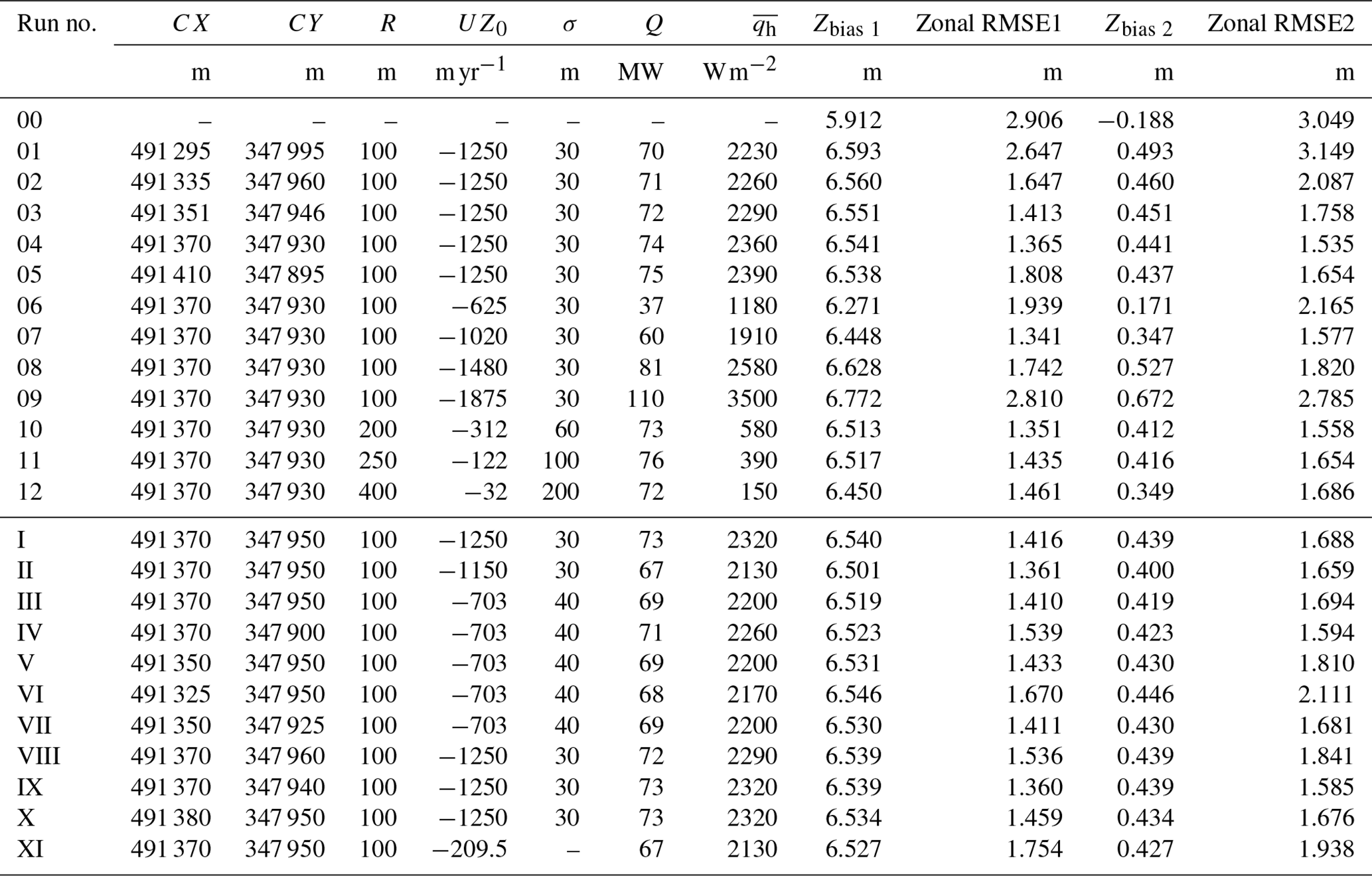
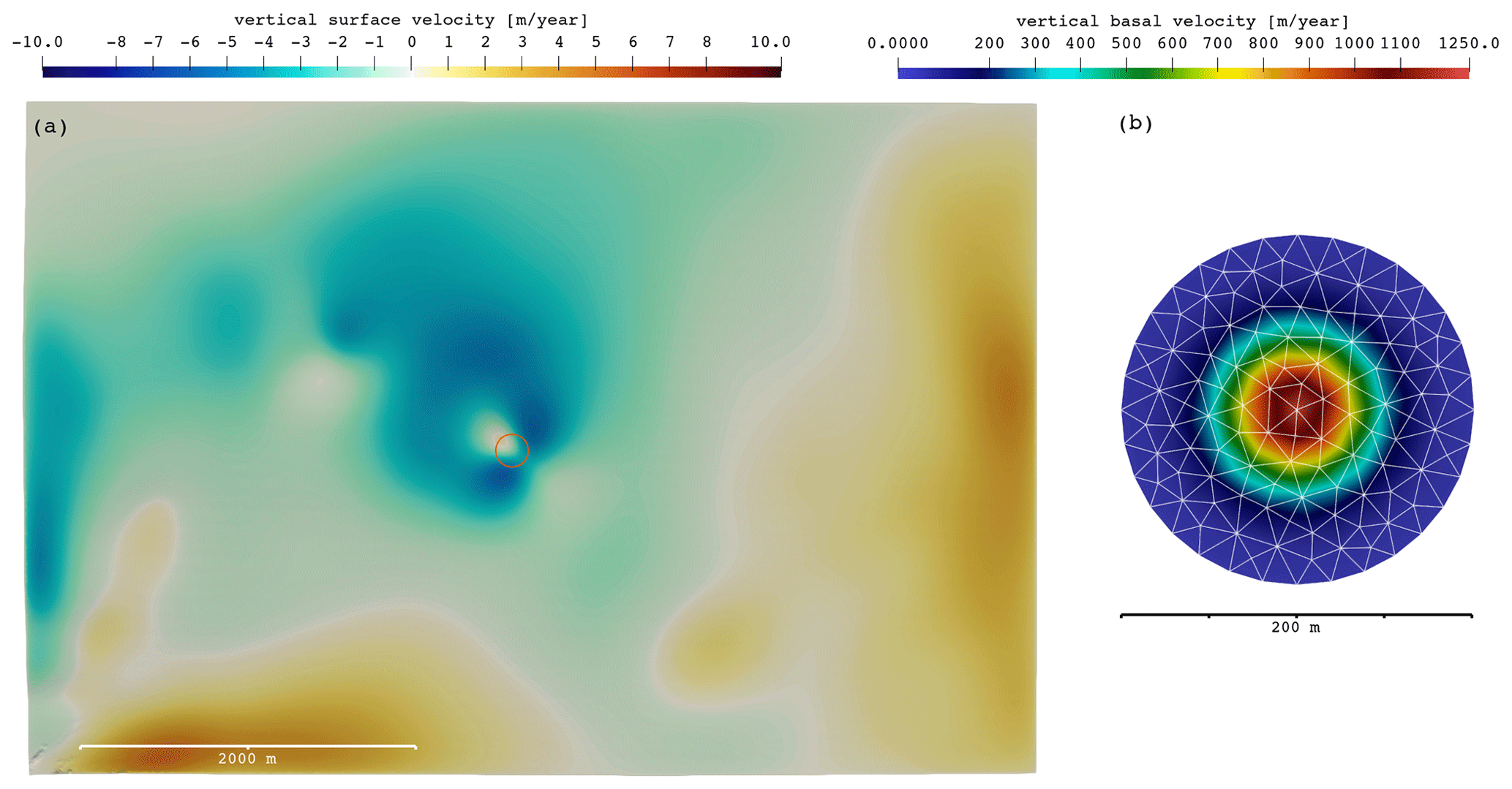
Figure 2(a) Vertical surface velocity field for run no. 04 over the whole model domain with a corresponding scale bar (cf. Fig. 1, red box). (b) The prescribed vertical basal outflow velocity distribution with its corresponding scale bar. The location and extent of this distribution are marked by the orange circle in panel (a).
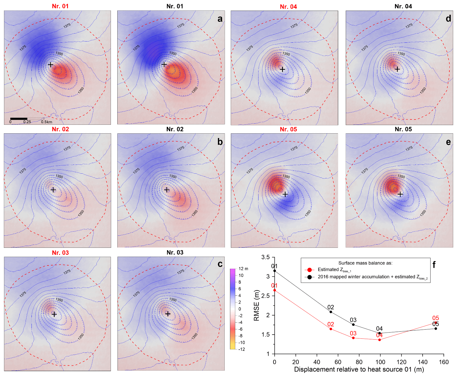
Figure 3(a–e) Image maps for the focus area of K6 (cf. dashed red square in Fig. 1), showing the difference between the simulated glacier surface HMcor and the observed glacier surface, H2017, with variable locations of heat source center (shown with a plus sign) beneath K6 (common color bar in panel c). The blue elevation contours (5 m interval) indicate the glacier surface in 2017. The numbers above indicate simulation number given in Table 1; red numbers refer to surface mass balance correction in Eq. (5), black numbers refer to surface mass balance correction in Eq. (6). (f) The RMSE calculated for the simulations in panels (a)–(e) within the boundary of the K6 (dashed red line in panels a–e).
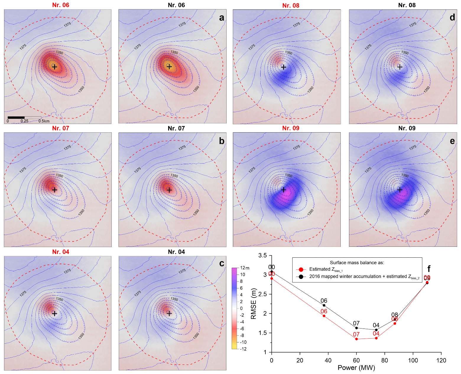
Figure 4(a–d) Image maps for the focus area of K6 (cf. dashed red square in Fig. 1), showing the difference between the simulated glacier surface HMcor and the observed glacier surface, H2017, with variable net power (Q) of the heat source beneath K6 (common color bar in panel c). Locations of heat source center are shown with a plus sign. The blue elevation contours (5 m interval) indicate the glacier surface in 2017. The numbers above indicate simulation number given in Table 1; red numbers refer to the surface mass balance correction in Eq. (5), black numbers refer to surface mass balance correction in Eq. (6). (f) The RMSE calculated within the boundary of the K6 (dashed red line in panels a–e) for the simulations in panels (a)–(e).
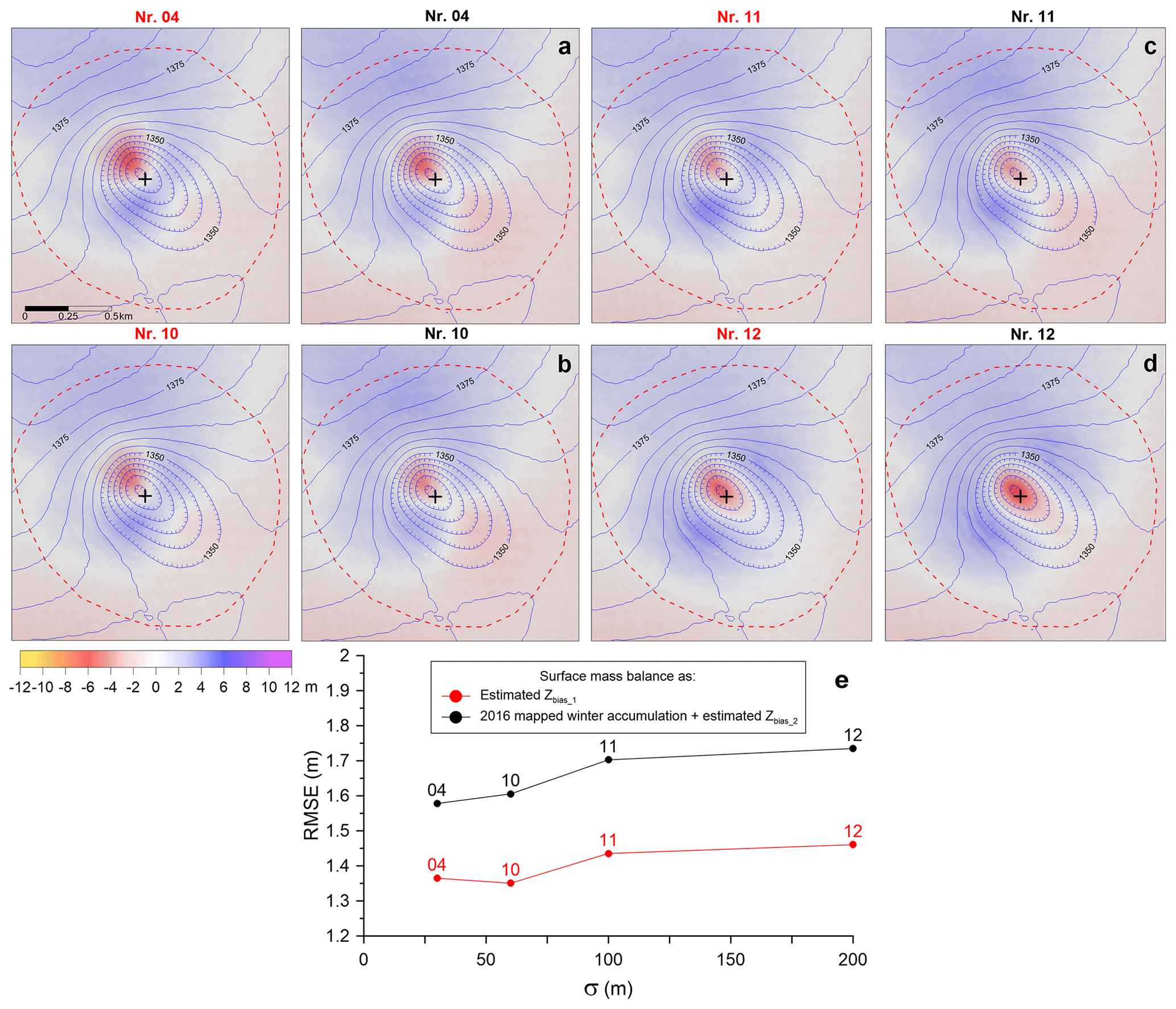
Figure 5(a–d) Image maps for the focus area of K6 (cf. dashed red square in Fig. 1), showing the difference between the simulated glacier surface HMcor and the observed glacier surface, H2017, with variable width (σ) of the heat source beneath K6 (common color bar below). Locations of heat source center is shown with a plus sign. The blue elevation contours (5 m interval) indicate the glacier surface in 2017. The numbers above indicate simulation number given in Table 1; red numbers refer to surface mass balance correction in Eq. (5), black numbers refer to the surface mass balance correction in Eq. (6). (e) The RMSE calculated within the boundary of the K6 (dashed red line in panels a–d) for the simulations in panels (a)–(d).
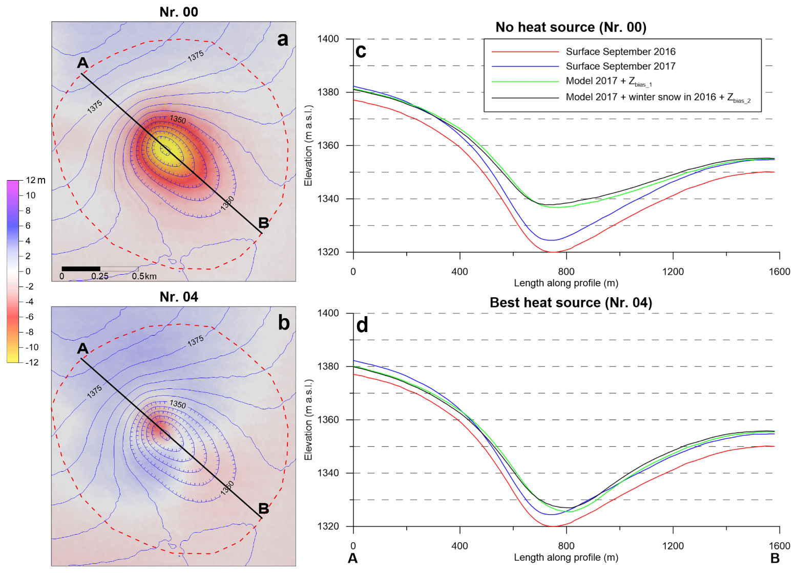
Figure 6(a, b) Image maps for the focus area of K6 (cf. dashed red square in Fig. 1) showing difference between the simulated glacier surface HMcor (spatially varying surface mass balance according to Eq. 6) and the observed glacier surface, H2017. (c, d) Center line elevation profile from A to B (location shown in panels a and b) of the glacier surface in September 2016 and 2017 compared with HMcor for the no heat source (c) and best-fit heat source (d). The green and black curves in panels (c)–(d) show the difference between assuming constant (Eq. 6) and variable winter snow distributions (Eq. 7).
An initial exploration of the parameter space for a possible subglacial heat flux distribution (i.e., ) has been carried out with 11 simulations (listed with Roman numerals as Run no. in Table 1). Based on these initial results, we have decided to continue the parameter search on a restricted parameter subspace that varies the heat source center (CX,CY) only along the center axis of the cauldron but continues to vary net power (Q) and heat source width (σ). This choice has been made as our initial simulations clearly have indicated that off-center axis heat source locations result in poor performance measures. Below, we detail the three optimization steps that have been used to further search the parameter space. Results are listed with Arabic numerals in Table 1:
- (I)
The heat source location. We set m yr−1, σ=30 m and R=100 m, resulting in Q of 70–75 MW, but due to the discretization of the heat source on the triangulated basal numerical grid, the integrated value of Q varies slightly with center location. These initial parameters were obtained from various simulation tests, considering the net power obtained for K5 and K6 in 2016–2017 in Jarosch et al. (2020). This heat source center was assumed to be located on a line forming an approximate mirror axis of the cauldron and moved it along this axis from northwest to southeast (Fig. 3 and runs 01–05 in Table 1).
- (II)
The net power, Q. Having established which location resulted in the best fit with reference data, simulations using the optimized location; σ=30 m; and m yr−1, −1020 m yr−1, −1480 m yr−1, −1875 m yr−1 (Fig. 4 and runs 06–09 in Table 1), and −1250 m yr−1 (run 04), corresponding to Q=37, 60, 81, 110, and 74 MW, were compared. Furthermore, a simulation showing the development of the cauldron with the heat source turned off beneath K5 and K6 (Fig. 6a and run 00 in Table 1) was carried out.
- (III)
The heat source width. Using the best center location of the heat source from (I), simulations were carried out using σ=30, 60, 100 and 200 m (Fig. 5 and runs 04 and 10–12 in Table 1), with corresponding values of R=100, 200, 250, and 400 m and , −312, −122, and −32 m yr−1, respectively. For all cases, this results in Q close to 75 MW (cf. Table 1).
In Table 1, we also report average basal heat fluxes () for the geothermal area, based on R. Even though some of our heat flux estimates are high (above 2000 W m−2), such high values have been reported for other geothermal areas in volcanic regions (e.g., Sorey and Colvard, 1994).
2.4 Surface mass balance and validation
After each ice flow simulation has been carried out (cf. Fig. 2), grid points at the ice surface are extracted and moved in 3D space according to Eq. (3). The surface datasets we use (cf. Sect. 2.1) are 339 d apart; thus, Δt=0.9281 years. Comparison with simulations carried out with a temporally high-resolution model (Wirbel and Jarosch, 2020) confirmed that in our application a one-time step evolution on a moving grid is entirely sufficient to represent the surface changes above the cauldrons. For all ice flow simulations, the 3D point cloud of surface points moved by the ice motion were gridded with bilinear interpolation to create 2D surface elevation maps (HM) with a horizontal resolution of 10×10 m. Including the effects of surface mass balance (cf. Eq. 2) results in
The surface mass balance within our focus area was not measured during the winter of 2016–2017. We therefore apply two different assumptions to estimate . The first one is assuming that is constant for a specific cauldron due to the relatively small area and elevation span (∼80 m for K6). This constant, referred to as Zbias 1, was estimated as the mean value of H2017−HM at the outlined cauldron boundary (shown in Figs. 3–6 for K6), resulting in
Snow radar measurements over the cauldrons of Mýrdalsjökull do, however, indicate significant variation in winter accumulation within the cauldrons (Hannesdóttir, 2021). A radar survey carried out in May 2016 showed a distinct pattern of accumulation in the cauldrons related to snow drift with ∼25 % increase in thickness, relative to the surroundings on the eastern side of the cauldron, i.e., the lee side to the governing wind direction carrying precipitation (easterly winds), while the western side of the cauldron opposing the easterly winds showed an ∼20 % reduction relative to the surroundings. These values correspond to ∼2.5 and ∼2.0 m, respectively, in ice equivalent. A snow radar survey repeated on fewer profiles in 2018 indicated a very similar pattern (Hannesdóttir, 2021). In our latter approach, we therefore assume that the effects due to redistribution of winter snow by snow drift are the same every year; therefore, we calculate
where bw2015−2016 is the snow thickness map surveyed with snow radar in May 2016 (Hannesdóttir, 2021), multiplied by 0.58 for conversion to ice, assuming a snow density of 530 kg m−3 (average value of surveyed snow density in mass balance snow cores obtained in the accumulation area of Mýrdalsjökull in May 2016) and an ice density of 917 kg m−3. The constant Zbias 2 was estimated as the mean value of at the outlined cauldron boundary. Applying this approach, it is assumed that the variations in winter accumulation from year to year as well as the summer mass balance can be treated spatially as a constant.
For both approaches used to correct for surface mass balance (Eqs. 6 and 7), we finally compute a domain-wide model error,
and extract E values within the borders of K5 and K6. After testing several performance measures (not presented here), we find zonal RMSE values to be very suitable in describing our model performance. The RMSE within the boundary of K5 was ∼0.8 m (applying Eq. 6) and ∼0.9 m (applying Eq. 7) for all runs with heat sources (simulation (sim.) 01–12), but its shape (see Sect. 2.3) and power (10 MW) were kept fixed beneath K5 for all of them. Given the relatively low power beneath K5, we considered it unrealistic to improve this crude approximation in our simulations; therefore, it is not considered further in this study.
During the study, various other simulations were carried out, including a simulation with constant outflow velocity instead of a Gaussian (Eq. 4) or center positions outside the central axis. The statistics of these simulations were found to be significantly worse than the optimal result from schemes (I)–(III) in terms of the RMSE and are thus omitted in this publication.
The results from our simulations are presented in Table 1 and Figs. 3–6. In general, both approaches applied to compensate for elevation changes caused by surface mass balance (Eqs. 6 and 7) yield similar results in terms of which parameters fit best. The fit with the validation data is highly dependent on the location of the heat source (Fig. 3). Simulation 01 (Fig. 3a), corresponding to a shift in the heat source center by 100 m northwest of the simulation with best fit in terms of RMSE (sim. 04, shown in Fig. 3d), results in comparable RMSE to the simulation with no heat source (sim. 00, shown in Fig. 6a). Simulation 03 (Fig. 3c), with heat source 25 m northwest of the 04 heat source, visually appears even better than sim. 04 (Fig. 3d), due to smaller maximum deviation from validation data, but it does however give slightly higher RMSE for both surface mass balance approaches (Fig. 3e). Moving the heat source southeast of the 04 heat source does, however, result in both higher RMSE and larger maximum errors (Fig. 3e–f). Simulations with heat source center locations shifted off the cauldron mirror axis (not shown here) result in worse RMSE for heat source center more than 20 m from the best fit source (sim. 04). When using the best fit location but varying Q, the best fits were obtained for sim. 07 (Q=60 MW) and sim. 04 (Q=74 MW). The RMSE values are quite similar in both cases; applying constant surface mass balance (Eq. 6) favors Q=60 MW, while applying variable surface mass (Eq. 7) favors Q=74 MW. Likely, the actual power is somewhere between these values.
Our results are the least dependent on the different shapes of heat source tested for approximately fixed Q and location (Fig. 5). For both approaches of estimating the effects of surface mass balance, there is barely a significant difference between using σ=30 m (Fig. 5a) and σ=60 m (Fig. 5b), both in terms of the RMSE (Fig. 5e) and visual comparison. The fit does however become significantly worse for σ=100 m, both for the RMSE and from visual comparison, revealing a stronger blue color in the sides of the cauldron, indicating modelled lowering that is too high (Fig. 5c). This becomes more pronounced for σ=200 m, which also results in the cauldron becoming too shallow as indicated by the darker red color in the cauldron center (Fig. 5d). When viewing the results of modelling validation, errors in the input glacier surface DEM in 2016, as well as the validation data consisting of the 2017 surface DEM and the estimated winter snow distribution, must be considered. The two DEMs cover around 190 km2 of common area ( of Mýrdalsjökull ice cap). If the difference between them is inspected, areas of similar size as the outlined area of K6 typically reveal a difference with ∼0.2 m standard deviation for smooth glacier surface, contributed by random high-frequency pixel noise on top of gradual variation in the difference. Such errors have minor effects on the validation and are also likely to be similar for the RMSE of all simulations, hardly shifting the values by more than 1–2 cm. The 2017 DEM was co-registered to the 2016 DEM to ensure that the elevation difference pattern caused by the horizontal shift between the DEMs was minimal. Shifting one DEM relative to the other by even just one pixel horizontally (4 m × 4 m) clearly increases slope/aspect-dependent differences between the DEMs. If we still assume that up to one pixel shift between the DEMs is possible and redo all RMSE calculations (for all simulation in Table 1), assuming variable surface mass balance (Eq. 7) and taking into account all combination of −4, 0 and 4 m horizontal shift in easting direction and −4, 0 and 4 m in the northing direction, then the minimum RMSE is obtained for simulation 04 in all cases except one, in which it gave the second lowest RMSE.
Summarizing the results of the model validations and the sensitivity check for possible errors in the validation data, we claim that the location of the heat source center is fairly well established, likely with ∼25 m location uncertainty. The heat source beneath K6 had a mean power of MW from autumn 2016 to autumn 2017, with the lower boundary corresponding to the best-fit value, when assuming spatially fixed surface mass balance (Eq. 6). The shape of the heat source distribution is the most uncertain quantity we infer. Simulations with significantly higher RMSE for σ≥100 m compared to σ≤60 m do, however, indicate that most of the heat at the ice–bed interface is released over a relatively small area ( m2), spanning less than 2 % of the 1.8 km2 cauldron area outlined with a dashed red line in Figs. 3–6.
The performance of our simulations, quantified by low zonal RMSE values, is highly sensitive to the location of the subglacial heat flux distribution. Shifting the heat source location by only 25 m (i.e., run 03 vs. 04) demonstrates clear changes in RMSE values, which highlights the need for high-resolution computational meshes to adequately model the effects of heat sources beneath ice cauldrons on ice dynamics and glacier surface changes. Even though we compute our results on a 20 m horizontal resolution grid, we are still able to pinpoint the location of the heat source with about the same level of accuracy. In contrast to observations from a GNSS station, operated at K6 in the summers of 2016 and 2017 (Fig. 1b), revealing seasonal water storage and drainage under the simulated cauldron, we assume continuous and instant water drainage underneath the glacier. This simplification is required for Eq. (1) to be applicable, as a persisting water body would substantially alter the heat transfer between the geothermal system and the ice. Our modelling approach utilizes the integrative nature of ongoing subglacial processes which all contribute to the observed annual glacier surface changes. Hence, by simulating nearly a complete year of glacier surface evolution, we are able to reproduce the accumulated mass changes within the system, even though we have simplified the surface evolution as such and the temporal nature of possible subglacial water storage changes.
Which heat source yields the best fit depends to some degree on how the effects of surface mass balance are estimated. This raises the question of which of the two approaches is more applicable. By comparison of the obtained bias corrections (Zbias 1 and Zbias 2) with existing surface mass balance data (unpublished data at Institute of Earth Sciences, University of Iceland) near K6, we can check how well these methods likely capture the average surface mass balance around K6. The value obtained for Zbias 1, used in Eq. (6), was for most simulations ∼6.5 m (Table 1), slightly lower than 7.2 m net mass balance (ice equivalent) measured at mass balance site M1, ∼2.5 km southeast of cauldron K6 (see Fig. 1a) from September 2016 to September 2017. The value obtained for Zbias 2, used in Eq. (7), was for most simulations ∼0.4 m (Table 1). During the summer of 2017, the ablation was measured at six sites at locations forming a cross shape over K6 (Fig. 1b). These measurements showed relatively low ablation of only 0.4–0.8 m with a mean value of 0.65 m (ice equivalent). If this was taken into account by adding the term with the summer ablation in 2017 to Eq. (7), then the value would become ∼1.1 m. This is in good agreement with measured winter mass balance at M1, yielding 1.2 m higher mass balance in the winter of 2016–2017 (7.8 mm ice equivalent) than in the winter of 2015–2016 (6.6 m ice equivalent) for which the snow was mapped in spring 2016 and used in Eq. (7).
The above comparison with surface mass balance data therefore suggests that, even though both approaches show fairly good agreement with existing surface mass balance data, a slightly better agreement is obtained when assuming a spatially varying surface mass balance, with the same spatial pattern as in spring 2016 (Eq. 7). However, when looking at the RMSE alone, it favors Eq. (6), which gives a lower best-fit RMSE (1.351 m for sim. 10) than Eq. (7) (RMSE =1.535 m for sim. 04). This may indicate that the pattern of winter accumulation caused by snow drift of the governing easterly wind directions was much less prominent in the winter 2016–2017 than in 2015–2016 and again in 2017–2018 (Hannesdóttir, 2021). Alternatively, the reason may be heat sources used in the simulations that are too simple, causing Eq. (6) to result in lower RMSE for the wrong reasons, whereas more complex heat sources such as a narrow line source or multiple Gaussian heat sources with different centers would give more optimal results with lower RMSE for Eq. (7). In the absence of better data to constrain the winter mass balance in 2016–2017, we do, however, consider further simulation to constrain more complex heat distribution at the bed to be non-conclusive.
This study highlights how fast steep depressions in a glacier surface, such as the ice cauldron K6, can be filled by ice flow in the absence of geothermal heat (Fig. 6a and c). With the heat source turned off beneath K6, our modelling indicates a reduction in depth of ∼15 m in a single year, from ∼45 to ∼30 m. This further demonstrates the precaution needed when linking reduced cauldron depth to water accumulation (Magnússon et al., 2021). In areas of powerful subglacial geothermal activity such as on Mýrdalsjökull, reduction in geothermal heat beneath a cauldron can result in similar depth changes as caused by subglacial water accumulation beneath cauldrons. If a lake formed beneath a glacier in the absence of strong geothermal heat source drains, creating a sharp depression in the glacier surface above as has been observed on the Greenland ice sheet, (e.g., Palmer et al., 2013), the ice dynamics are bound to play a significant role in filling up the depression following the lake drainage.
In this contribution, we have demonstrated an efficient modelling approach to quantify subglacial heat source locations, distributions and heat fluxes. Even though we apply simplifications to subglacial melt processes as well as surface mass balance, we are able to locate subglacial heat sources accurately to the resolution of our computational grid. The methods applied focus on the overall mass changes within the system integrated over almost a whole year, which is sufficient to adequately quantify heat fluxes, despite not resolving seasonal variations. Our best fitting model (run 04) infers a Gaussian-shaped heat source distribution under K6, resulting in a total heat flux of MW. In combination with the configuration used at K5 (Q=10 MW), we get a total heat flux output at K5 and K6 combined of MW. This result agrees well with previous estimates of MW (Jarosch et al., 2020). Additionally, we show that the area of the main heat source beneath K6 in 2016 to 2017 was <0.03 km2, which is less than 2 % of the areal extent of the resulting ice surface depression (∼1.8 km2).
The method presented here is not only suitable to indirectly measure geothermal heat fluxes below glaciers and ice-sheets, but it also has great potential for continuously monitoring subglacial geothermal systems and estimating their risk potential for infrastructure as well as humans.
All ice flow simulations in this contribution have been carried out with the well-established Elmer/Ice software package (Gagliardini et al., 2013).
The 2016 and 2017 surface DEMs, the bedrock DEM, and the simulation-based 2017 surface data for our best fitting simulation (run no. 04) can be accessed from a dedicated Zenodo repository (https://doi.org/10.5281/zenodo.11185656, Jarosch et al., 2024).
AHJ carried out all simulations presented, preformed the simulation data analysis and contributed to writing. AHJ and EM designed the study experiment. EM carried out the comparison of data simulations and observed elevation changes, contributed to writing, and produced all figures, except Fig. 2. KH processed and analyzed the snow radar data. JMCB processed the DEMs extracted from Pléiades data in 2016 and 2017. FP analyzed in situ surface mass balance data and processed GNSS data used in this study. FP and JMCB reviewed the manuscript and contributed to discussions on its content.
The contact author has declared that none of the authors has any competing interests.
Publisher's note: Copernicus Publications remains neutral with regard to jurisdictional claims made in the text, published maps, institutional affiliations, or any other geographical representation in this paper. While Copernicus Publications makes every effort to include appropriate place names, the final responsibility lies with the authors.
Pléiades images used to produce surface DEMs were acquired at a subsidized cost thanks to the CNES ISIS program. Sveinbjörn Steinþórsson, Ágúst Þór Gunnlaugsson and Bergur Einarsson as well as JÖRFÍ volunteers are thanked for their work during field trips.
This research has been supported by Rannís (grant no. 163391).
This paper was edited by Adam Booth and reviewed by Fausto Ferraccioli and two anonymous referees.
Belart, J. M. C., Magnússon, E., Berthier, E., Gunnlaugsson, Á. Þ., Pálsson, F., Aðalgeirsdóttir, G., Jóhannesson, T., Thorsteinsson, T., and Björnsson, H.: Mass Balance of 14 Icelandic Glaciers, 1945–2017: Spatial Variations and Links With Climate, Front. Earth Sci., 8, 163, https://doi.org/10.3389/feart.2020.00163, 2020. a, b
Björnsson, H.: Hydrology of ice caps in volcanic regions, University of Iceland, 1988. a
Björnsson, H. and Pálsson, F.: Icelandic glaciers, Jökull, 58, 365–386, 2008. a
Björnsson, H., Pálsson, F., and Guðmundsson, M. T.: Surface and bedrock topography of the Mýrdalsjökull ice cap, Iceland: The Katla caldera, eruption sites and routes of jökulhlaups, Jökull, 49, 29–46, 2000. a
Dziadek, R., Ferraccioli, F., and Gohl, K.: High geothermal heat flow beneath Thwaites Glacier in West Antarctica inferred from aeromagnetic data, Commun. Earth Environ., 2, 162, https://doi.org/10.1038/s43247-021-00242-3, 2021. a
Gagliardini, O., Zwinger, T., Gillet-Chaulet, F., Durand, G., Favier, L., de Fleurian, B., Greve, R., Malinen, M., Martín, C., Råback, P., Ruokolainen, J., Sacchettini, M., Schäfer, M., Seddik, H., and Thies, J.: Capabilities and performance of Elmer/Ice, a new-generation ice sheet model, Geosci. Model Dev., 6, 1299–1318, https://doi.org/10.5194/gmd-6-1299-2013, 2013. a, b
Guðmundsson, M. T. and Högnadóttir, Þ.: Upptök og stærð jökulhlaups í Múlakvísl niðurstöður flugmælinga, Memo, 2011. a
Guðmundsson, M. T., Högnadóttir, Þ., Kristinsson, A. B., and Guðbjörnsson, S.: Geothermal activity in the subglacial Katla caldera, Iceland, 1999–2005, studied with radar altimetry, Ann. Glaciol., 45, 66–72, https://doi.org/10.3189/172756407782282444, 2007. a
Hannesdóttir, K.: Estimating snow accumulation on Mýrdalsjökull and Öræfajökull with snow radar using Discrete Gabor Transform for image analysis. Implications to the mass balance of ice cauldrons, mathesis, Faculty of Earth Sciences, University of Iceland, 2021. a, b, c, d
Jarosch, A. H. and Gudmundsson, M. T.: Numerical studies of ice flow over subglacial geothermal heat sources at Grímsvötn, Iceland, using Full Stokes equations, J. Geophys. Res., 112, F02008, https://doi.org/10.1029/2006jf000540, 2007. a, b, c
Jarosch, A. H., Magnússon, E., Wirbel, A., Belart, J. M. C., and Pálsson, F.: The geothermal output of the Katla caldera estimated using DEM differencing and 3D iceflow modelling, Tech. rep., RH-02-20, Zenodo [data set], https://doi.org/10.5281/ZENODO.3784657, 2020. a, b, c, d, e
Jarosch, A. H., Magnússon, E., and Belart, J. M. C.: Geothermal heat source estimations through ice flow modelling at Mýrdalsjökull, Iceland – Datasets (1.0), Zenodo [data set], https://doi.org/10.5281/zenodo.11185656, 2024. a
Jóhannesson, T., Björnsson, H., Magnússon, E., Guðmundsson, S., Pálsson, F., Sigurðsson, O., Thorsteinsson, T., and Berthier, E.: Ice-volume changes, bias estimation of mass-balance measurements and changes in subglacial lakes derived by lidar mapping of the surface Icelandic glaciers, Ann. Glaciol., 54, 63–74, https://doi.org/10.3189/2013AoG63A422, 2013. a
Jóhannesson, T., Pálmason, B., Hjartarson, Á., Jarosch, A. H., Magnússon, E., Belart, J. M. C., and Gudmundsson, M. T.: Non-surface mass balance of glaciers in Iceland, J. Glaciol., 66, 685–697, https://doi.org/10.1017/jog.2020.37, 2020. a, b
Kundu, P. K., Cohen, I. M., and Dowling, D. R.: Fluid Mechanics, Elsevier, https://doi.org/10.1016/c2012-0-00611-4, 2016. a
Larsen, G., Guðmundsson, M. T., and Sigmarsson, O.: Náttúruvá á Íslandi, chap. Katla, 211–233, Viðlagatrygging Íslands Háskólaútgáfan, ISBN 978-9979-54-943-7, 2013. a
Magnússon, E., Pálsson, F., Jarosch, A. H., van Boeckel, T., Hannesdóttir, H., and Belart, J. M. C.: The bedrock and tephra layer topography within the glacier filled Katla caldera, Iceland, deduced from dense RES-survey, Jökull, 71, 39–70, https://doi.org/10.33799/jokull2021.71.039, 2021. a, b, c, d, e, f, g, h
Magnússon, E., Pálsson, F., Guðmundsson, M. T., Belart, J. M. C., and Högnadóttir, Þ.: Hvað sýna íssjármælingar undir sigkötlum Mýrdalsjökuls, Tech. rep., Institute of Earth Sciences, University of Iceland, 2017. a
Palmer, S. J., Dowdeswell, J. A., Christoffersen, P., Young, D. A., Blankenship, D. D., Greenbaum, J. S., Benham, T., Bamber, J., and Siegert, M. J.: Greenland subglacial lakes detected by radar, Geophys. Res. Lett., 40, 6154–6159, https://doi.org/10.1002/2013gl058383, 2013. a
Shean, D. E., Alexandrov, O., Moratto, Z. M., Smith, B. E., Joughin, I. R., Porter, C., and Morin, P.: An automated, open-source pipeline for mass production of digital elevation models (DEMs) from very-high-resolution commercial stereo satellite imagery, ISPRS J. Photogramm. Remote, 116, 101–117, https://doi.org/10.1016/j.isprsjprs.2016.03.012, 2016. a, b
Sigurðsson, O., Zóphóníasson, S., and Ísleifsson, E.: Jökulhlaup úr Sólheimajökli 18. júlí 1999, Jökull, 49, 75–80, 2000. a
Smith-Johnsen, S., de Fleurian, B., Schlegel, N., Seroussi, H., and Nisancioglu, K.: Exceptionally high heat flux needed to sustain the Northeast Greenland Ice Stream, The Cryosphere, 14, 841–854, https://doi.org/10.5194/tc-14-841-2020, 2020a. a
Smith-Johnsen, S., Schlegel, N.-J., Fleurian, B., and Nisancioglu, K. H.: Sensitivity of the Northeast Greenland Ice Stream to Geothermal Heat, J. Geophys. Res.-Earth Surf., 125, e2019JF005252, https://doi.org/10.1029/2019jf005252, 2020b. a
Sorey, M. L. and Colvard, E. M.: Measurements of heat and mass flow from thermal areas in Lassen Volcanic National Park, California, 1984-93, Tech. Rep. 94-4180, U.S. Geological Survey, 1994. a
Winsborrow, M. C., Clark, C. D., and Stokes, C. R.: What controls the location of ice streams?, Earth-Sci. Rev., 103, 45–59, https://doi.org/10.1016/j.earscirev.2010.07.003, 2010. a
Wirbel, A. and Jarosch, A. H.: Inequality-constrained free-surface evolution in a full Stokes ice flow model (evolve_glacier v1.1), Geosci. Model Dev., 13, 6425–6445, https://doi.org/10.5194/gmd-13-6425-2020, 2020. a, b
Þórarinsson, S. and Rist, S.: Rannsókn á Kötlu og Kötluhlaupi sumarið 1955, Jökull, 5, 43–46, 1955. a