the Creative Commons Attribution 4.0 License.
the Creative Commons Attribution 4.0 License.
 | 03 May 2024
Experimental modelling of the growth of tubular ice brinicles from brine flows under sea ice
Sergio Testón-Martínez
Laura M. Barge
Jan Eichler
C. Ignacio Sainz-Díaz
Julyan H. E. Cartwright
We present laboratory experiments on the growth of a tubular ice structure surrounding a plume of cold brine that descends under gravity into water with a higher freezing point. Brinicles are geological analogues of these structures found under sea ice in the polar regions on Earth. Brinicles are hypothesized to exist in the oceans of other celestial bodies, and being environments rich in minerals, serve a potentially analogous role as an ecosystem on icy-ocean worlds to that of submarine hydrothermal vents on Earth.
- Article
(3718 KB) - Full-text XML
- BibTeX
- EndNote


Ice brinicles are tubular, finger-like formations that grow downwards from the underside of sea ice into the underlying seawater (Cartwright et al., 2013). They are formed when pockets of concentrated salt brine in the sea ice are released (Weissenberger et al., 1992), causing a plume of cold, dense brine to flow downward from the bottom of the ice layer into the surrounding seawater. As the brine descends, the temperature difference between the brine (which, owing to freezing point depression, may reach as low as −23 °C while remaining liquid) and the seawater (near its freezing point, ∼ −1.8 °C) leads to the formation of a hollow tube of ice around the brine that can extend several metres down into the ocean, even sometimes reaching the seafloor (Fig. 1). In the earlier literature, ice brinicles were also called “ice stalactites” (Paige, 1970; Martin, 1974; Dayton and Martin, 1971; Perovich et al., 1995), but an icicle is an ice stalactite that has a different growth mechanism than a brinicle, so we argue against the use of that term. Brinicles have been found in both the Arctic and Antarctic oceans (Katlein et al., 2020; BBC, 2011) and are of interest due to their potential role in the transport of heat, salt, and other materials between the ocean and the atmosphere (Cartwright et al., 2013). Brinicles also share morphological similarities with other self-assembling structures, in particular with chemical gardens (Barge et al., 2015). Both types of structures exhibit tubular, finger-like morphology and can extend several centimetres to several metres in length, and brinicles have been described as an unusual example of an inverted chemical garden (Fig. 2; Cartwright et al., 2013; Pampalakis, 2016). Additionally, both structures are examples of self-organizing systems that exhibit complex dynamical behaviour (Cartwright et al., 2013).
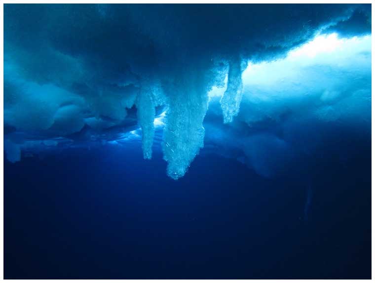
Figure 1Brinicles filmed under sea ice near McMurdo Station in Antarctica. Image courtesy of Rob Robbins, US Antarctic Program.
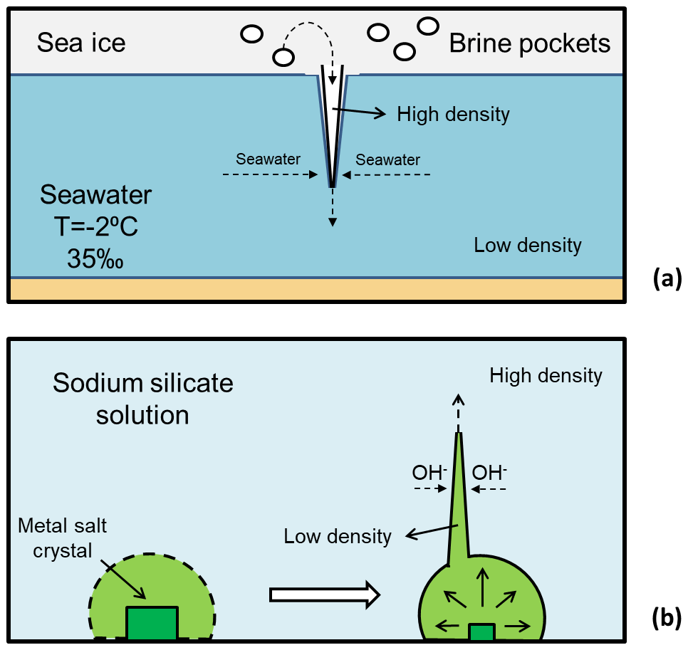
Figure 2(a) Diagram of the formation of a brinicle, illustrating how the brine is ejected downwards from sea ice and freezes the seawater, forming a tubular ice structure. (b) Diagram of the formation of a chemical garden, illustrating the creation of the garden membrane as well as its rupture and tubular growth.
The study of brinicles dates back several decades, with early research focused on their formation, structure, and dynamics. Field observations from Antarctica have been reported since the 1970s (Paige, 1970; Dayton and Martin, 1971; Perovich et al., 1995; BBC, 2011). The first laboratory study from 1974 used a combination of experiments and theoretical models to investigate the formation and growth of brinicles in seawater (Martin, 1974). Martin found that the inner and outer brinicle radius increases with time and noted that the interior flow is convectively unstable and controls the brinicle tip radius. Also, as determined by Martin (1974), only a fraction of the ice formed actually contributes to forming the brinicle, and most ice crystals are swept out into the surrounding seawater. Since brinicles inject cold brine beneath the ice layer, they may be relevant to ice sheet desalination and upper-ocean mixing (Perovich et al., 1995; Dayton and Martin, 1971). It is important to consider the potential biological and ecological impacts of ice brinicles, as microbial communities have been discovered in hypersaline brines (Bougouffa et al., 2013; Steinle et al., 2018). Brinicles may also form in extraterrestrial environments and affect ocean mixing and microenvironments on other celestial bodies, for example, under the ice shell of Jupiter's moon Europa (Vance et al., 2019; Buffo et al., 2021a).
Although significant progress has been made in understanding the formation and dynamics of brinicles, there is still much to be learned about these structures, in particular, what conditions lead to their formation and what effects variations in these conditions (growth velocity, morphology, and microstructure of the precipitates) have on their formation. In this study, we created brinicles in the laboratory using different methods in order to study the conditions under which they might form on Earth and on other worlds.
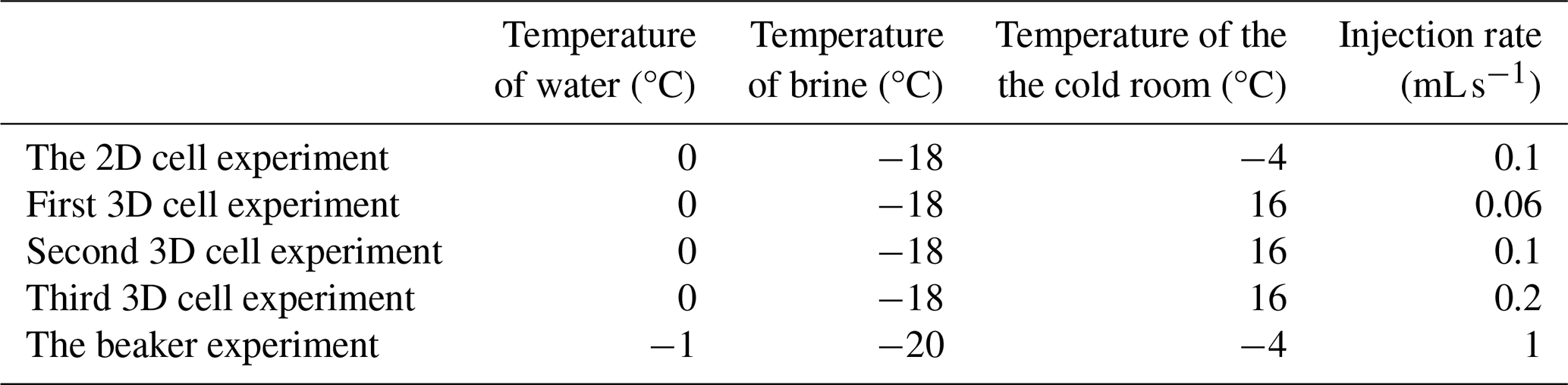
Three different experimental methods were used to attempt to grow brinicles in the laboratory, injecting a cold brine flow into a reservoir of less-salty water. We varied the size of the reservoir in which the brine flow occurred as well as the injection rate and aperture (Table 1).
The first method, “2D-cell”, used a Hele-Shaw cell (54 mm×54 mm) formed by two methacrylate walls with 1 mm of separation between them, as has been used in previous studies to create chemical gardens confined in two dimensions (Rocha et al., 2021; Ding et al., 2016; Haudin et al., 2014). The second method, “3D cell”, also used a similar Hele-Shaw cell but with a larger (10 mm) separation between the methacrylate walls. We should also note saline water freezing experiments in a Hele-Shaw cell by Niedrauer and Martin (1979) and Middleton et al. (2016). The brine was composed of a 25 % weight solution of NaCl in tap water chilled in a −24 °C freezer until completely frozen. Then it was taken out and left defrosting in a −4 °C freezer for 2 h before injection. The Hele-Shaw cell or beaker was filled with cold tap water at ∼ 0 °C. In the 2D cell and 3D cell experiments, the brine at ∼ −18 °C was injected by hand using a 10 mL syringe through a 0.9 mm gauge needle at approximately 0.06, 0.1, or 0.2 mL s−1. These values were determined by dividing the volume injected by the total time of the experiment. The 2D and 3D cell experiments were conducted in a cold room at 4 °C, while some of the 3D cell experiments were also carried out at 16 °C. We also tried to inject the brine using a syringe pump, which offers greater control over the injection rate. However, this was unsuccessful since the ∼ 0.3 m of tubing needed to connect the syringe to the Hele-Shaw cell facilitated too much heat transfer to the brine, even when insulated using packing wrap, such that upon injection the temperature was no longer low enough for a brinicle to form. Experiments were monitored by filming with a Nikon D3400 digital single-lens reflex (DSLR) camera set up 20 cm from the Hele-Shaw cells. For the 3D cell experiment, we also studied the formation of the structures with a schlieren optics setup, as was used in previous studies of salt fingers (Linden, 1973) and sea ice applications (Middleton et al., 2016). The same camera and a blue laser were used to witness fluid flow during brinicle formation.
The third method, “beaker”, used a larger (3 L) rectangular glass container. It was initially filled with 2 L H2O + 3.5 % mass fraction of NaCl (seawater analogue) cooled down to −1 °C. The brine was a saturated NaCl solution cooled down to −20 °C. The brine was injected using a hose with a diameter of 3 mm with a valve to adjust the flow rate, which was important in order to initiate the brinicle growth that started when flow was established. The flow rate was estimated considering that 1 L of brine typically took 15–20 min to flow through the system. The experiments were performed in a cold room at 4 °C. The brine container and the tubing were thermally insulated using foam material. Experiments were monitored by filming with a Nikon D3400 DSLR camera set up 20 cm from the experiment. Different setups were tried; in later runs a second tube was added to remove the brine from the bottom of the beaker. In that way, we were able to reduce mixing of seawater and brine and maintain relatively constant salinity of the seawater. As a result, using this setup the brinicle grew until reaching the bottom of the container.
Table 1Experimental data of the temperatures of the water, brine, and cold room used for each experiment in degrees Celsius, as well as the brine injection rates for each method.
The 3D cell and beaker experiments formed brinicles, and these were further analysed using photographs taken throughout the experiments. For the 3D cell experiments at the three injection rates, we measured the total length of the brinicle, the thickness of the brinicle at the top part touching the injection needle, and the diameter of the lowest point of the brinicle every 5 s. With the beaker experiments, videos of brinicle growth were used to make measurements of the same parameters every 5 s.
3.1 Laboratory brinicle formation
The 2D Hele-Shaw cell method with 1 mm separation, which we have used previously to form injection chemical gardens of various chemistries (Haudin et al., 2014), did not lead to brinicle formation because the cell width was too narrow for ice tube growth. The narrow separation between the cell walls only facilitated a 2D brine flow structure rather than a cylinder as in the 3D experiments. As shown in Fig. 3, upon brine injection the seawater surrounding the brine flow began to freeze and formed a closed ice structure around the needle and brine, impeding the creation of a 3D brinicle. Instead, the brine touched the walls and caused ice formation in all directions. After some time, more brine could not be injected because it was obstructed by ice (see movie S1 in https://doi.org/10.20350/digitalCSIC/15364, Testón-Martínez et al., 2023).
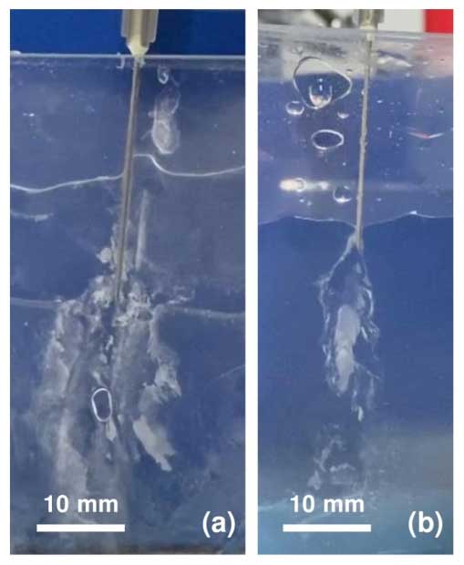
Figure 3Two brinicle experiments 10 s after injection (a) and (b), following the 2D cell method with a 1 mm separation between the cell walls. In both cases solid instead of tubular ice structures were formed. See movieS1 in https://doi.org/10.20350/digitalCSIC/15364 (Testón-Martínez et al., 2023).
The 3D cell method formed brinicles, and details of the fluid flows could be observed with a schlieren setup. With a greater separation between walls (10 mm), the self-clogging phenomenon observed in the 2D cell method did not occur, and a tubular ice structure formed (Fig. 4; see movieS2 in https://doi.org/10.20350/digitalCSIC/15364, Testón-Martínez et al., 2023). As the brine started to flow into the cell, it sank toward to the bottom due to the density difference, and freezing was observed starting from the top of the brine flow as the brinicle width and length increased with time. Ice also formed around the brine injection needle because it was colder than the reservoir. Shortly after the start of the injection, the ice wall that formed around the brine flow was very thin, as can be observed in Fig. 5b; the ice wall thickened over the course of the injection (Fig. 5c). Eventually, the brinicle reached the bottom of the cell (Fig. 5d), and the brine flow began to accumulate at the bottom forming a bi-layer system with a high-density brine phase and water phase while continuing to freeze at the water–brine interface. This formed a brine layer capped by an ice layer in the lower part of the cell, making the deposited ice layer grow thicker (Fig. 5e; see movieS3 in https://doi.org/10.20350/digitalCSIC/15364, Testón-Martínez et al., 2023). When the brinicle reached the bottom, the growth of the brine phase caused the hollow brinicle walls to expand and form a bell-shaped tube.
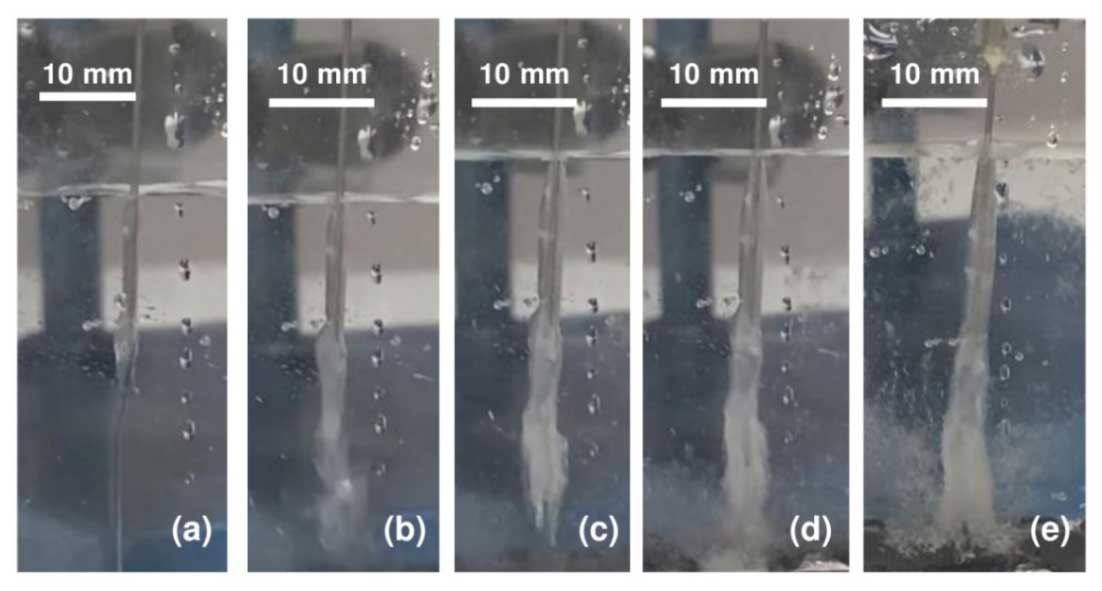
Figure 4Evolution of a brinicle created with the 3D cell method. (a) Start of the injection and freezing of the flow walls (00:03.13; timestamp format is minutes:seconds). (b) Downward freezing of the brinicle (00:10.10). (c) Widening of the brine flow walls (00:13.13). (d) The brinicle reaches the bottom of the cell (00:16). (e) Freezing of the “seafloor” (00:19.35). See movieS2 in https://doi.org/10.20350/digitalCSIC/15364 (Testón-Martínez et al., 2023).
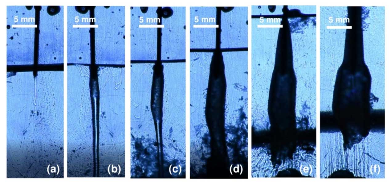
Figure 5Evolution of a brinicle created with the 3D cell method and filmed with a schlieren optical setup. (a) Start of the injection (00:00). (b) Initial freezing of the brine flow walls (00:07.12). (c) Downwards freezing of the brinicle walls (00:10.80). (d) Freezing at the bottom of the cell and release of ice particles (00:20). (e) Breakdown of the brinicle and ice layer deposition at the interface (00:48.48). (f) After the injection was stopped, melting of the deposited ice and reshaping of the brinicle (01:15.68). See movieS3 in https://doi.org/10.20350/digitalCSIC/15364 (Testón-Martínez et al., 2023).
After stopping the injection (Fig. 5f), we observe how the brinicle melts, with pieces of ice breaking off. A series of upward flows are observed due to dilution or freshening of the system (Fig. 5f). Moreover, the fluid interface (black band in Fig. 5e) separating the high-density phase with the salt concentration from the lighter water phase was tested, and the insertion of a temperature probe into this interface (Fig. 6) revealed that temperatures varied in different areas of the cell. Above the interface it was 0.6 °C and below the interface (Fig. 6b) it was −1.5 to −3 °C, whereas the interface itself (Fig. 6a) had a temperature of approximately 0 °C. In Fig. 6 we can also see that the interface (highlighted with a yellowish colour created with a light set) remained stable when being touched by the temperature probe; only after stirring the solution thoroughly with the probe did this band disappear.
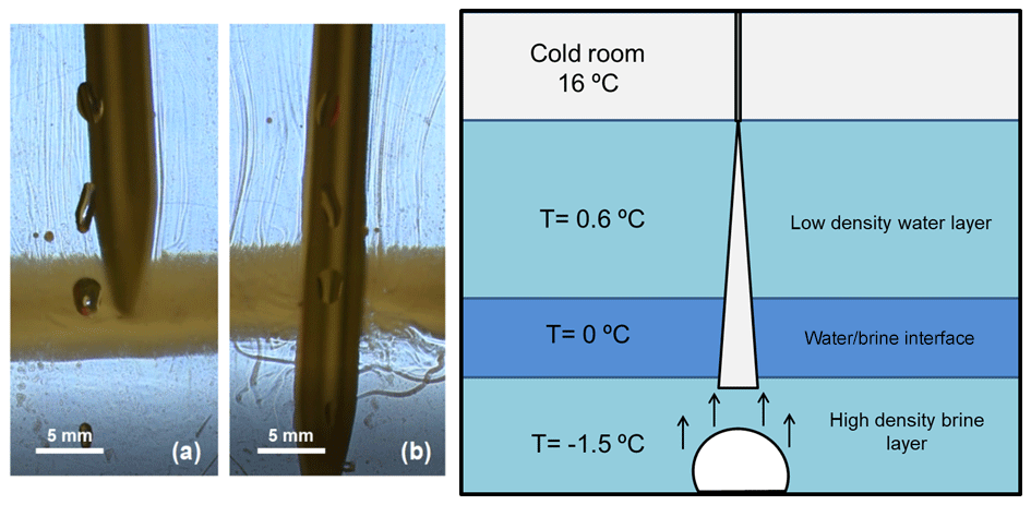
Figure 6Photography and sketch of the interface created during the 3D Hele-Shaw cell experiment in Fig. 5. The schlieren method was used to observe the movement of the fluids when interacting with a temperature probe (a) above the brine–water interface and (b) below it. The yellow colour of the interface is a highlighting optic effect created with a light set.
The beaker method also formed brinicles, which were larger than those created in the 3D cell method. Figure 7 shows the formation of a brinicle in the beaker experiment. The brine flow from the hose (Fig. 7a) starts to freeze from the top (Fig. 7b) and continues to freeze the brine flow walls (Fig. 7c) while widening its diameter (Fig. 7d) until it reaches the bottom of the container (Fig. 7e; see movieS4 in https://doi.org/10.20350/digitalCSIC/15364, Testón-Martínez et al., 2023). The completed brinicle had textured ice walls that appeared porous, as seen in the image in Fig. 8. In the larger brinicles formed in the beaker experiment, we observed that on the outer edges of the brinicle horizontally oriented ice crystals were visible (Fig. 9); this was also observed in photos of brinicles from Antarctica (Fig. 9) where the initial ice crystals also grew perpendicular to the brine flow. These crystals are probably oriented normal to the c axis along the a axis, known to be the fastest growth direction in ice (Glen and Perutz, 1954).
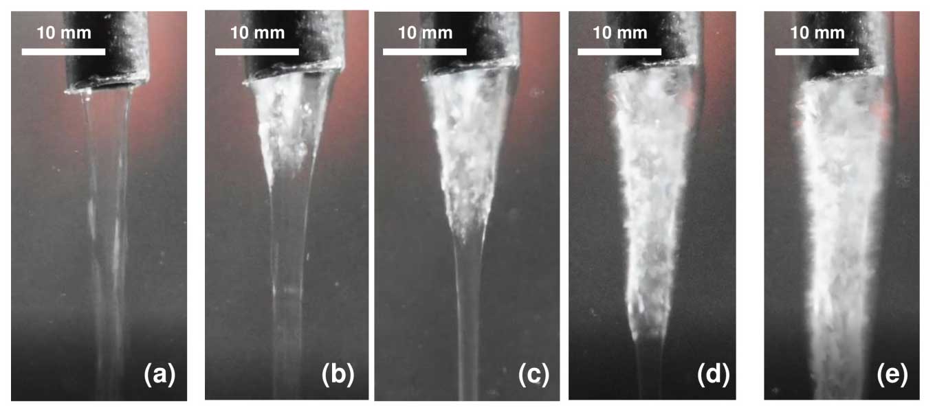
Figure 7Evolution of a brinicle created with the beaker method. (a) Start of injection (00:00). (b) Start of freezing of the brinicle walls (00:07.91). (c) Downwards freezing of the brine flow (00:14.45). (d) Widening of the brinicle over time (00:40.21). See movieS4 in https://doi.org/10.20350/digitalCSIC/15364 (Testón-Martínez et al., 2023).
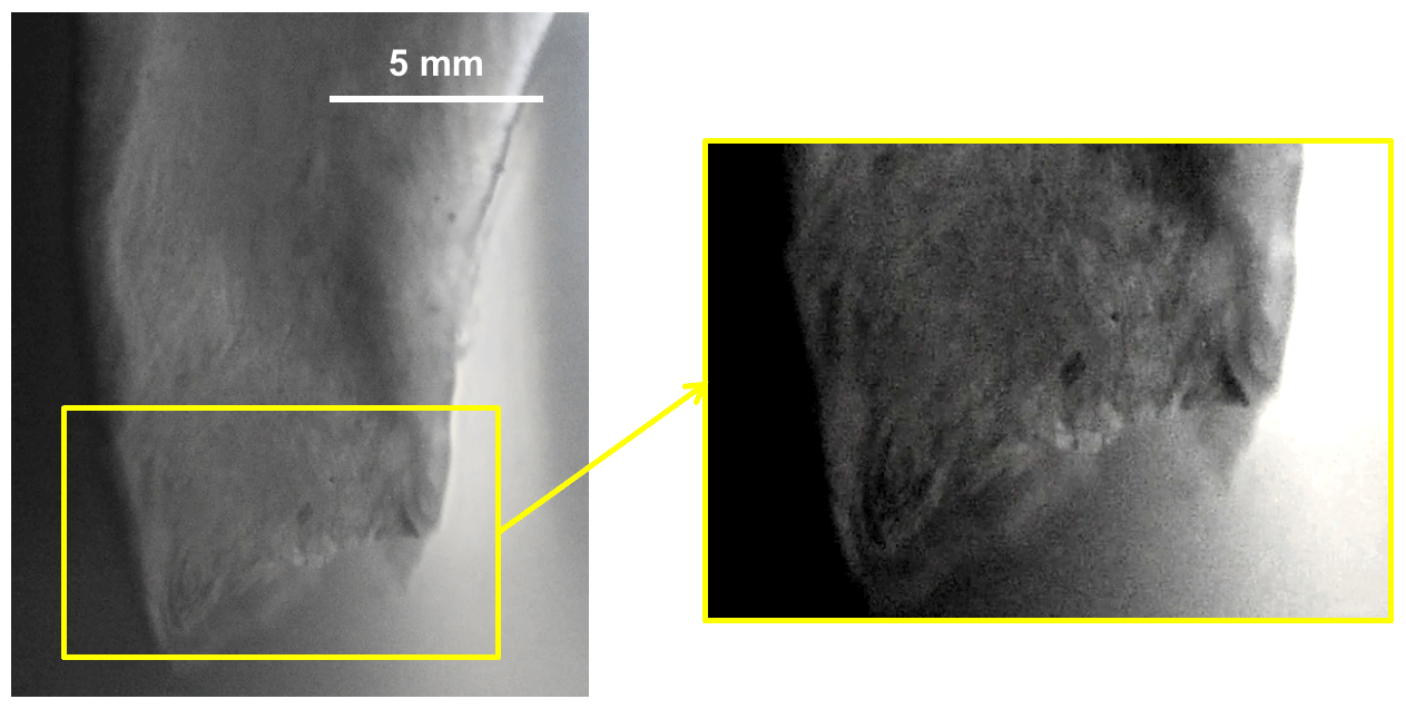
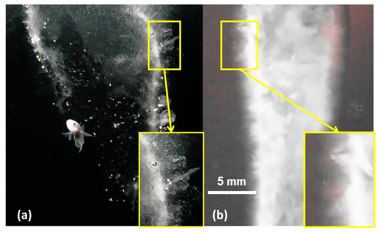
Figure 9Comparison between the walls of (a) a brinicle found near McMurdo Station in Antarctica and (b) a brinicle made in the laboratory using the beaker method. In both structures, horizontally oriented crystals perpendicular to the brinicle wall can be seen. Image (a) is courtesy of Rob Robbins, US Antarctic Program. An approximate scale for (a) is provided by the fish.
In all experiments, once brinicles formed they were very fragile; it was not possible to physically extract them from the experiments, and if the needle or hose was moved, they would quickly disaggregate.
3.2 Physical analysis of brinicle growth
In the 3D cell experiments, the brinicle growth velocities calculated by measuring the change in the brinicle height every 5 s decreased over time, and moreover, brinicles grew more slowly at lower brine injection rates (Fig. 10a). These data fit the model from Martin (1974), who analysed brinicle growth in terms of a Graetz problem – the fluid mechanics of tube flow that couples fluid flow with heat transfer – since brinicle growth is proportional to the square root of time. As the brinicle length increases with time, the brine that arrives at the lowest point is not as cold as the initial brine injected because it receives heat from the surroundings. This makes the freezing of the brinicle and consequent growth more difficult than at the start.
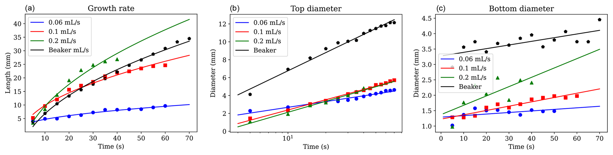
Figure 10Measurements over time of (a) brinicle growth rate, (b) brinicle diameter at the brine injection point, and (c) brinicle diameter at the bottom. The first three lines represent a 3D cell experiment with different brine flow rates: 0.06 mL s−1 (blue), 0.1 mL s−1 (red), and 0.2 mL s−1 (green), while the last one (black) used the beaker method. The fit in panel (a) is proportional to the square root of time (Martin, 1974). An error of ∼ 1 % (10 µm) comes from the distance measuring program. Note that the last points in each series represent the brinicle touching the bottom of the container, causing the points not to follow the expected fit. See movieS5 and movieS6 in https://doi.org/10.20350/digitalCSIC/15364 (Testón-Martínez et al., 2023).
The widening of the brinicles at the starting point was observed to slow down with time (Fig. 10b), probably due to the brinicle walls being too thick at some point to facilitate further freezing on the outside of the wall. We chose to measure the top of the brinicle that touched the needle because it was frozen from the start so the widening was more obvious. All the experiments at different injection rates have a similar tendency in width increase, indicating that this widening is independent of the brine flux.
Figure 10c represents the diameter of the lowest point of the brinicle at each time point. As shown in Fig. 4, the brinicle walls grow thicker with time; this is reflected in the observation that the lowest diameter of a brinicle also becomes wider as the brinicle grows. To confirm this, we also measured the brinicle width at one of the lowest points for a time lapse (at the same brinicle height) after its creation, and we found that it follows the same tendency shown in Fig. 10b where its width increase grows and then slows down. The flux of brine also affects this behaviour, as seen in Fig. 10c where the experiments with higher flux have faster growth than the ones with lower flux. The oscillations visible in the curves imply an oscillatory growth instability that warrants further investigation. This may be related to the periodic popping regime observed in chemical gardens (Barge et al., 2015; Thouvenel-Romans and Steinbock, 2003).
The brinicle formed in the beaker experiment (Fig. 7) was measured similarly using one of the videos (see movieS4 in https://doi.org/10.20350/digitalCSIC/15364, Testón-Martínez et al., 2023) and showed similar behaviour to the brinicles in the 3D cell experiments (Fig. 4). Brinicle growth velocity decreases with time (Fig. 10a) while the width of the brinicle at the injection point increases until it becomes stable (Fig. 10b), and the thickness of the lowermost part of the brinicle increases with time (Fig. 10c).
Brinicles and chemical gardens are both instances of fluid-jet-templated tube growth; they differ in that brinicles grow by thermal diffusion, which is approximately 100× faster than the chemical diffusion in chemical gardens (Cardoso and Cartwright, 2017). Nevertheless, the same physical model can be employed. This shows that the tube radius should vary with flow rate following the Poiseuille flow driven by a pressure gradient, , and a density difference, Δρig (Cardoso and Cartwright, 2017),
where R is the radius and μi the viscosity. This is shown in Fig. 11.
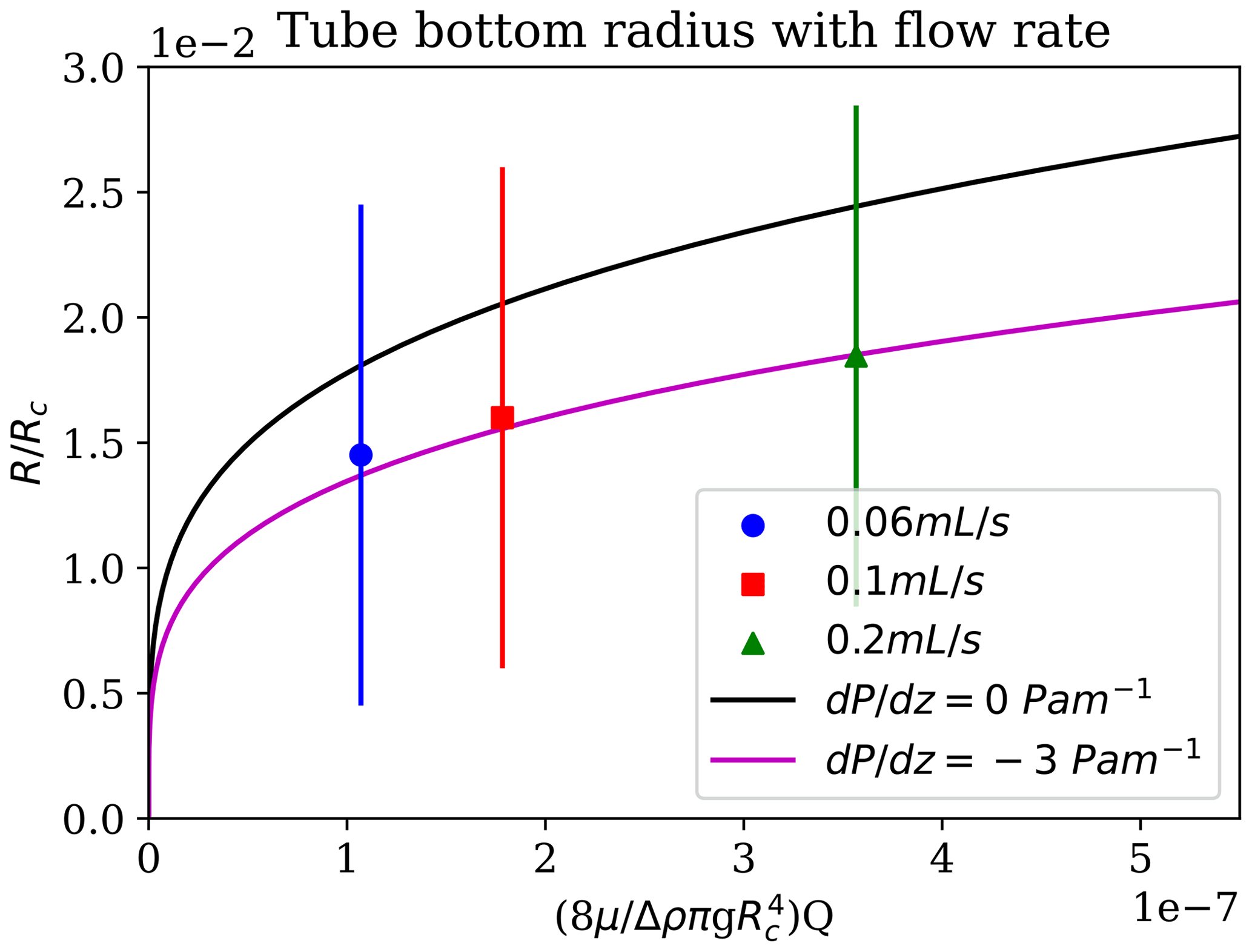
Figure 11Brinicle measurements of the radius at the bottom of the brinicle at the same time for different flow rates. The three points represent a 3D cell experiment with different brine flow rates: 0.06 mL s−1 (blue), 0.1 mL s−1 (red), and 0.2 mL s−1 (green). The first fit line (black) represents the prediction from the Poiseuille flow (Cardoso and Cartwright, 2017) if Pa m−1 and the second if Pa m−1. An error of ∼ 1 % (10 µm) comes from the distance measuring programme. See movieS5 and movieS6 in https://doi.org/10.20350/digitalCSIC/15364 (Testón-Martínez et al., 2023).
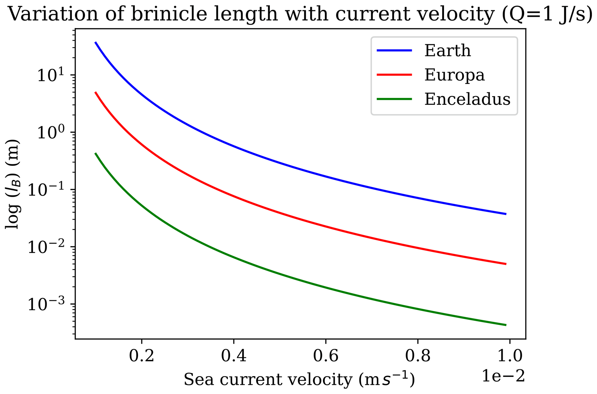
Figure 12Brinicle length calculated using the scaling length for a buoyant plume in a cross flow (Eq. 2) for different sea current velocities. The length has been calculated using general parameters for Earth (blue), Europa (red), and Enceladus (green) for a fixed value, Qh, of the heat flux in the plume.
Growth of brinicles in a laboratory setting is highly dependent on the parameters of the experimental setup, each of which reflects particular aspects of a natural brinicle system. In this work, the most high-fidelity analogues to natural brinicles were formed in a large glass container with brine fed through a hose; in the smaller, more controlled Hele-Shaw cell systems, a larger separation between the walls than was needed in previous work was required to witness brinicle growth. This is consistent with other experimental studies that have used similar setups to grow ice. In previous studies, Hele-Shaw cells with 2–3 mm separation have been used to grow ice and form brine channels, in which planar freezing fronts but no brinicles were observed, even when brine channels formed (Middleton et al., 2015; Eide and Martin, 1975).
In our 1 mm 2D cell experiment, we also observed freezing fronts that touched the cell walls, but this separation was too narrow to permit ice tube formation. The size and shape of the brine flow aperture are also important as they determine the initial brinicle diameter (Fig. 10) as well as the brine flow rate. In a natural system, where brine flow into seawater is the result of many connected brine pockets and channels within the ice (Weissenberger et al., 1992), the radius of the brine channel draining into the seawater below would not be constant, as in our experiments where needles and hoses are used, but would adjust to the brine flow rate as more buoyant seawater intrudes up into the neck and freezes, until the forces of seawater buoyancy and brine pressure are balanced (Eide and Martin, 1975). In our experiments, the injection rate (0.06–0.2 mL s−1), which takes the place of the force of brine pressure, is still lower than estimated brine flow rates in natural brinicles, ∼ 1 to 16 mL s−1, reported by Perovich et al. (1995) and Dayton and Martin (1971), respectively, dictated by the amount of brine flowing downward from underneath the sea ice.
Temperature is a crucial parameter, since for brinicles to form, seawater must be near its freezing point (≤ 1.8 °C), while the brine temperature must be much lower (< −15 °C). A rise in temperature in either fluid or both fluids makes brinicle formation impossible as the seawater does not get cold enough to freeze. This was one of the lessons learned in our cell experiments. The use of a syringe pump would be preferred in terms of controlling the experimental parameters; however, the requirement of tubing to connect the syringe to the cell led to too much temperature change in the brine before it contacted the water reservoir. To optimize the flow rate and injection aperture position while maintaining the sub-freezing brine temperature, the whole experiment should be done with a syringe pump in a cold room.
Brinicles grow relatively quickly. In our experiments, brinicles centimetres to tens of centimetres long formed in minutes, which is comparable to growth speeds witnessed in geological environments; natural brinicle growth speeds have been reported from ∼ 0.2 to 2 cm min−1 (Perovich et al., 1995; Dayton and Martin, 1971). The size, spacing, and internal structures of brinicles can vary as well depending on their growth conditions. Both small (10–100 cm long; Paige, 1970) and large (1–6 m long, 5–25 cm wide; Dayton and Martin, 1971; Perovich et al.; 1995, Paige, 1970) brinicles have been observed in McMurdo Sound, Antarctica. The brinicles in our 2D cell experiments appear to have one single channel (Fig. 5) due to brine injection from a single narrow injection point, although we were not able to remove them from the experimental apparatus to analyse their internal structure. However, in natural systems, brinicles can be more heterogeneous in structure; e.g. Perovich et al. (1995) reported a brinicle from Antarctica that had five separate internal sub-channels. Brinicles occur alone or in groups, but they occur sparsely (∼ 5–10 m spacing between them; Paige, 1970; Perovich et al., 1995). This is because there is a minimum amount of seawater necessary to generate the concentrated brine (estimated 10 L seawater per L of brine; Cartwright et al., 2013), and, depending on the size of the brinicle and the brine channel from which it formed, Dayton and Martin (1971) and Perovich et al. (1995) estimated 130 and 70 L of brine, respectively, were needed to grow the brinicles that were observed in the field.
The extent to which brinicles could be relevant for the origin of life and for astrobiology (Vance et al., 2019; Cartwright et al., 2013; Buffo et al., 2021b; Howell and Leonard, 2023; Lawrence et al., 2023; Howell et al., 2024) would depend on how long they could persist on Earth or other planetary ocean–ice interfaces. Modelling studies have suggested that brinicles could form under the ice shell on Jupiter's moon Europa and that their lifetime would be dependent on the ice shell thickness – giving a range of hours to years (Buffo et al., 2021a), which encompasses the lifetimes of brinicles in terrestrial systems (e.g. in Antarctica, brinicles can persist for months; Dayton and Martin, 1971). Saturn's moon Enceladus also has a subsurface ocean and putative hydrothermal activity, and its plumes offer the opportunity to sample the subsurface ocean (Hsu et al., 2015; Postberg et al., 2009). It is possible that brinicles could form on Enceladus as well, although as yet there is no published modelling on brinicles in an Enceladus context.
Brinicles are initially fragile, and in our experiments, we observed that moving the injector after the experiment caused the brinicle to disaggregate. Similar fragility has been described for brinicles in the field that disintegrated when touched by a remotely operated vehicle arm (Perovich et al., 1995), although in that study they were able to recover the top 750 cm of a brinicle for analysis. Other brinicles were described as, “fragile but flexible enough to bend slightly with gentle tidal currents” (Paige, 1970). The lifetime of a brinicle would therefore depend on the currents, which would affect the stability of structure of the brine plume under the ice. Brinicles photographed under the Antarctic ice are often long and thin; they are high-aspect-ratio tubes. They are fragile, easily broken off, and – the argument goes (Buffo et al., 2021a) – would break off with larger currents or would be prevented from forming at all due to dispersion of the brine plume and so would not be of importance in an icy-world ocean. But brinicles are not always so long and thin; for example, the central one in Fig. 1 is short and wide. If a brine stream descends from sea ice into a lateral ambient current, it will have a different form to a plume in a quiescent fluid medium (Slawson and Csanady, 1967; Hewett et al., 1971). Hewett et al. (1971) discuss the basic scaling length for a buoyant plume in a cross flow, which they term the buoyancy length (lB),
where Qh is the heat flux in the plume, g is the gravitational acceleration, ρiCp is the heat capacity per unit volume of effluent fluid (i.e. the outflowing brine), T is the temperature of the ambient fluid (i.e. the ocean), and v is the cross-flow speed. lB is approximately the radius of curvature near the stack exit of a buoyant plume of negligible initial momentum. This gives a first-order estimate of the length a brinicle might grow to in a cross-flow situation.
Figure 12 shows this behaviour for brinicles on Earth as well as on Europa and Enceladus, two icy-ocean moons. The buoyancy length of a plume, and thus of a brinicle, decreases fast, with the cube of the speed of a transverse current. A brinicle in this environment on an icy world might look something like some seafloor hydrothermal vents that form in places with ambient currents. The ice making up such a brinicle would probably become more massive and less porous as the structure ages, somewhat similar to how snow falling on Earth gradually forms firn and then ice under ageing processes (Bartels-Rausch et al., 2012). Brinicles on Earth occur in a range of environments including shallow waters (e.g. BBC, 2011) but have also been observed in water up to 300 m deep (Dayton and Martin, 1971) and have been observed occurring far from land in the Arctic (Katlein et al., 2020). Therefore, we propose that brinicles may exist in some form even with currents in icy-world oceans. Since brinicles represent sites of high thermal and chemical gradients at the ice–ocean interface, they could be of interest as locations that might provide energy to support prebiotic chemistry or life (Vance et al., 2019; Cartwright et al., 2013). Further studies of these fascinating ice–brinicle systems may shed light on the conditions that are required for their formation in different ocean–ice chemistries and for their possible stability and lifetime on Earth and on other celestial bodies.
All data used in the paper, as well as the supplementary videos, are available at https://doi.org/10.20350/digitalCSIC/15364 (Testón-Martínez et al., 2023).
The supplementary videos are available at https://doi.org/10.20350/digitalCSIC/15364 (Testón-Martínez et al., 2023).
-
movieS1_2D_cell.mp4. This is a movie of the growth of brinicles in a 2D Hele-Shaw cell. The brine injection rate is 0.1 mL s−1. The water freezes in all directions.
-
movieS2_3D_cell.mp4. This is a movie of the growth of brinicles in a 3D Hele-Shaw cell. The brine injection rate is 0.1 mL s−1. A tubular ice structure (brinicle) is formed.
-
movieS3_3D_Schlieren.mp4. This is a movie of the growth of brinicles in a 3D Hele-Shaw cell using the schlieren optics technique. The brine injection rate is 0.1 mL s−1. Water, brine, and ice flows can be seen. The brinicle grows until freezing the bottom; then the flow stops.
-
movieS4_Baker.mp4. This is a movie of the growth of brinicles in a 3D beaker reactor. The brine injection rate is 1 mL s−1. The brine freezes the water, creating a brinicle that grows downwards and sideways.
-
movieS5_3D_cell_0,1mls.mp4. This is a movie of the growth of brinicles in a 3D Hele-Shaw cell. The brine injection rate is 0.1 mL s−1. The water around the needle freezes and a brinicle starts to grow downwards. Lower speed and diameter than with higher flows are observed.
-
movieS6_3D_cell_0,2mls.mp4. This is a movie of the growth of brinicles in a 3D Hele-Shaw cell. The brine injection rate is 0.2 mL s−1. The water around the needle freezes and a brinicle starts to grow downwards. Higher speed and diameter than with lower flows are observed.
All authors contributed in an integrated fashion to this work.
The contact author has declared that none of the authors has any competing interests.
Publisher's note: Copernicus Publications remains neutral with regard to jurisdictional claims made in the text, published maps, institutional affiliations, or any other geographical representation in this paper. While Copernicus Publications makes every effort to include appropriate place names, the final responsibility lies with the authors.
We thank Rob Robbins for providing the Antarctica brinicle photographs, which have not been previously published. Laura M. Barge was supported by the Jet Propulsion Laboratory (JPL) Topical Research & Technology Development and the NASA Presidential Early Career Award for Scientists and Engineers (PECASE). Laura M. Barge's research was carried out at the Jet Propulsion Laboratory, California Institute of Technology, under a contract with NASA (80NM0018D0004). The authors would like to acknowledge the contribution of the European Cooperation in Science and Technology (COST) Action CA17120 supported by the EU Framework Programme Horizon 2020. Sergio Testón-Martínez acknowledges the CSIC and Spanish Andalusian “Garantiìa Juvenil” project AND21_IACT_M2_ 058.
This research has been supported by the Consejería de Economía, Innovación, Ciencia, y Empleo, Junta de Andalucía (grant no. AND21_IACT_M2_058) and the National Aeronautics and Space Administration (grant no. 80NM0018D0004).
The article processing charges for this open-access publication were covered by the CSIC Open Access Publication Support Initiative through its Unit of Information Resources for Research (URICI).
This paper was edited by Jari Haapala and reviewed by Sönke Maus and one anonymous referee.
Barge, L. M., Cardoso, S. S. S., Cartwright, J. H. E., Cooper, G. J. T., Cronin, L., De Wit, A., Doloboff, I. J., Escribano, B., Goldstein, R. E., Haudin, F., Jones, D. E. H., Mackay, A. L., Maselko, J., Pagano, J. J., Pantaleone, J., Russell, M. J., Sainz-Díaz, C. I., Steinbock, O., Stone, D. A., Tanimoto, Y., and Thomas, N. L.: From Chemical Gardens to Chemobrionics, Chem. Rev., 115, 8652–8703, https://doi.org/10.1021/acs.chemrev.5b00014, 2015.
Bartels-Rausch, T., Bergeron, V., Cartwright, J. H., Escribano, R., Finney, J. L., Grothe, H., Gutiérrez, P. J., Haapala, J., Kuhs, W. F., Pettersson, J. B., and Price, S. D.: Ice structures, patterns, and processes: A view across the icefields, Rev. Mod. Phys., 84, 885, https://doi.org/10.1103/RevModPhys.84.885, 2012.
BBC: Finger of death. BBC Frozen Planet (Winter), https://www.bbc.co.uk/programmes/p00mq92j (last access: 23 November 2011), 2011.
Bougouffa, S., Yang, J., Lee, O., Wang, Y., Batang, Z. B., Al-Suwailem, A. M., and Qian, P.: Distinctive Microbial Community Structure in Highly Stratified Deep-Sea Brine Water Columns, Appl. Environ. Microb., 79, 3425–3437, https://doi.org/10.1128/aem.00254-13, 2013.
Buffo, J. J., Meyer, C. R., and Parkinson, J. R. G.: Dynamics of a solidifying icy satellite shell, J. Geophys. Res.-Planets, 126, e2020JE006741, https://doi.org/10.1029/2020JE006741, 2021a.
Buffo, J. J., Schmidt, B. E., Huber, C., and Meyer, C. R.: Characterizing the ice-ocean interface of icy worlds: A theoretical approach, Icarus, 360, 114318, https://doi.org/10.1016/j.icarus.2021.114318, 2021b.
Cardoso, S. S. S. and Cartwright, J. H. E.: On the differing growth mechanisms of black-smoker and Lost City-type hydrothermal vents, Proc. Roy. Soc. A-Math. Phy., 473, 20170387, https://doi.org/10.1098/rspa.2017.0387, 2017.
Cartwright, J. H. E., Escribano, B., González, D. L., Sainz-Díaz, C. I., and Tuval, I.: Brinicles as a Case of Inverse Chemical Gardens, Langmuir, 29, 7655–7660, https://doi.org/10.1021/la4009703, 2013.
Dayton, P. K. and Martin, S.: Observations of ice stalactites in McMurdo Sound, Antarctica, J. Geophys. Res., 76, 1595–1599, https://doi.org/10.1029/JC076i006p01595, 1971.
Ding, Y., Batista, B., Steinbock, O., and Cardoso, S. S. S.: Wavy membranes and the growth rate of a planar chemical garden: Enhanced diffusion and bioenergetics, P. Natl. Acad. Sci. USA, 113, 9182–9186, https://doi.org/10.1073/pnas.1607828113, 2016.
Eide, L. I. and Martin, S.: The formation of brine drainage features in young sea ice, J. Glaciol., 14, 137–153, https://doi.org/10.3189/S0022143000013460, 1975.
Glen, J. W. and Perutz, M. F.: The growth and deformation of ice crystals, J. Glaciol., 2, 397–403, 1954.
Haudin, F., Cartwright, J. H. E., Brau, F., and De Wit, A.: Spiral precipitation patterns in confined chemical gardens, P. Natl. Acad. Sci. USA, 111, 17363–17367, https://doi.org/10.1073/pnas.1409552111, 2014.
Hewett, A., Fay, J. A., and Hoult, D. P.: Laboratory experiments of smokestack plumes in a stable atmosphere, Atmos. Environ., 5, 767–772, https://doi.org/10.1016/0004-6981(71)90028-X, 1971.
Howell, S. M. and Leonard, E. J.: Ocean Worlds: Interior Processes and Physical Environments, in: Handbook of Space Resources, Springer International Publishing, Cham, 873–906, https://doi.org/10.1007/978-3-030-97913-3_26, 2023.
Howell, S. M., Bierson, C. J., Kalousová, K., Leonard, E., Steinbrügge, G., and Wolfenbarger, N.: Jupiter's ocean worlds: Dynamic ices and the search for life, in: Ices in the Solar-System, Elsevier, 283–314, https://doi.org/10.1016/B978-0-323-99324-1.00003-1, 2024.
Hsu, H.-W., Postberg, F., Sekine, Y., Shibuya, T., Kempf, S., Horányi, M., Juhász, A., Altobelli, N., Suzuki, K., Masaki, Y., Kuwatani, T., Tachibana, S., Sirono, S.-i., Moragas-Klostermeyer, G., and Srama, R.: Ongoing hydrothermal activities within Enceladus, Nature, 519, 207–210, https://doi.org/10.1038/nature14262, 2015.
Katlein, C., Mohrholz, V., Sheikin, I., Itkin, P., Divine, D. V., Stroeve, J., Jutila, A., Krampe, D., Shimanchuk, E., Raphael, I., Rabe, B., Kuznetsov, I., Mallet, M., Liu, H., Hoppmann, M., Fang, Y.-C., Dumitrascu, A., Arndt, S., Anhaus, P., Nicolaus, M., Matero, I., Oggier, M., Eicken, H., and Haas, C.: Platelet ice under Arctic pack ice in winter, Geophys. Res. Lett., 47, e2020GL088898, https://doi.org/10.1029/2020GL088898, 2020.
Lawrence, J. D., Mullen, A. D., Bryson, F. E., Chivers, C. J., Hanna, A. M., Plattner, T., Spiers, E. M., Bowman, J. S., Buffo, J. J., Burnett, J. L., and Carr, C. E.: Subsurface science and search for life in ocean worlds, The Planetary Science Journal, 4, 22, https://doi.org/10.3847/PSJ/aca6ed, 2023.
Linden, P.: On the structure of salt fingers, Deep Sea Research and Oceanographic Abstracts, 20, 325–340, https://doi.org/10.1016/0011-7471(73)90057-0, 1973.
Martin, S.: Ice stalactites: comparison of a laminar flow theory with experiment, J. Fluid Mech., 63, 51, https://doi.org/10.1017/s0022112074001017, 1974.
Middleton, C. A., Thomas, C., Escala, D. M., Tison, J.-L., and De Wit, A.: Imaging the Evolution of Brine Transport in Experimentally Grown Quasi-two-dimensional Sea Ice, Proc. IUTAM, 15, 95–100, https://doi.org/10.1016/j.piutam.2015.04.014, 2015.
Middleton, C. A., Thomas, C., De Wit, A., and Tison, J. L.: Visualizing brine channel development and convective processes during artificial sea-ice growth using schlieren optical methods, J. Glaciol., 62, 1–17, https://doi.org/10.1017/jog.2015.1, 2016.
Niedrauer, T. M. and Martin, S.: An experimental study of brine drainage and convection in young sea ice, J. Geophys. Res., 84, 1176–1186, 1979.
Paige, R. A.: Stalactite Growth beneath Sea Ice, Science, 167, 171–172, https://doi.org/10.1126/science.167.3915.171.b, 1970.
Pampalakis, G.: The Generation of an Organic Inverted Chemical Garden, Chem.-Eur. J., 22, 6779–6782, https://doi.org/10.1002/chem.201504773, 2016.
Perovich, D. K., Richter-Menge, J. A., and Morison, J. H.: The formation and morphology of ice stalactites observed under deforming lead ice, J. Glaciol., 41, 305–312, https://doi.org/10.3189/S0022143000016191, 1995.
Postberg, F., Kempf, S., Schmidt, J., Brilliantov, N., Beinsen, A., Abel, B., Buck, U., and Srama, R.: Sodium salts in E-ring grains from an ocean below the surface of Enceladus, Nature, 459, 1098–1101, https://doi.org/10.1038/nature08046, 2009.
Rocha, L. A. M., Cartwright, J. H. E., and Cardoso, S. S. S.: Filament dynamics in planar chemical gardens, Phys. Chem. Chem. Phys., 23, 5222–5235, https://doi.org/10.1039/D0CP03674A, 2021.
Slawson, P. and Csanady, G.: On the mean path of buoyant, bent-over chimney plumes, J. Fluid Mech., 28, 311–322, https://doi.org/10.1017/S0022112067002095, 1967.
Steinle, L., Knittel, K., Felber, N., Casalino, C. E., De Lange, G. J., Tessarolo, C., Stadnitskaia, A., Damsté, J. S. S., Zopfi, J., Lehmann, M. F., Treude, T., and Niemann, H.: Life on the edge: active microbial communities in the Kryos MgCl2-brine basin at very low water activity, ISME J., 12, 1414–1426, https://doi.org/10.1038/s41396-018-0107-z, 2018.
Testón-Martínez, S., Barge, L. M., Eichler, J., Sainz-Díaz, C. I., and Cartwright, J. H. E.: Experimental modelling of the growth of tubular ice brinicles from brine flows under sea ice, DIGITAL.CSIC [video], https://doi.org/10.20350/digitalCSIC/15364, 2023.
Thouvenel-Romans, S. and Steinbock, O.: Oscillatory growth of silica tubes in chemical gardens, J. Am. Chem. Soc., 125, 4338–4341, https://doi.org/10.1021/ja0298343, 2003.
Vance, S. D., Barge, L. M., Cardoso, S. S., and Cartwright, J. H.: Self-Assembling Ice Membranes on Europa: Brinicle Properties, Field Examples, and Possible Energetic Systems in Icy Ocean Worlds, Astrobiology, 19, 685–695, https://doi.org/10.1089/ast.2018.1826, 2019.
Weissenberger, J., Dieckmann, G., Gradinger, R., and Spindler, M.: Sea ice: A cast technique to examine and analyze brine pockets and channel structure, Limnol. Oceanogr., 37, 179–183, https://doi.org/10.4319/lo.1992.37.1.0179, 1992.