the Creative Commons Attribution 4.0 License.
the Creative Commons Attribution 4.0 License.
 | 22 Aug 2022
Halving of Swiss glacier volume since 1931 observed from terrestrial image photogrammetry
Erik Schytt Mannerfelt
Amaury Dehecq
Romain Hugonnet
Elias Hodel
Matthias Huss
Andreas Bauder
Daniel Farinotti
The monitoring of glaciers in Switzerland has a long tradition, yet glacier changes during the 20th century are only known through sparse observations. Here, we estimate a halving of Swiss glacier volumes between 1931 and 2016 by mapping historical glacier elevation changes at high resolution. Our analysis relies on a terrestrial image archive known as TerrA, which covers about 86 % of the Swiss glacierised area with 21 703 images acquired during the period 1916–1947 (with a median date of 1931). We developed a semi-automated workflow to generate digital elevation models (DEMs) from these images, resulting in a 45 % total glacier coverage. Using the geodetic method, we estimate a Swiss-wide glacier mass balance of −0.52 ± 0.09 m w.e. a−1 between 1931 and 2016. This equates to a 51.5 ± 8.0 % loss in glacier volume. We find that low-elevation, high-debris-cover, and gently sloping glacier termini are conducive to particularly high mass losses. In addition to these glacier-specific, quasi-centennial elevation changes, we present a new inventory of glacier outlines with known timestamps and complete attributes from around 1931. The fragmented spatial coverage and temporal heterogeneity of the TerrA archive are the largest sources of uncertainty in our glacier-specific estimates, reaching up to 0.50 m w.e. a−1. We suggest that the high-resolution mapping of historical surface elevations could also unlock great potential for research fields other than glaciology.
- Article
(11312 KB) - Full-text XML
- BibTeX
- EndNote


Glaciers are melting rapidly on a global scale, and constraints on regional- to global-scale volume changes since the 2000s have been constantly improving (Gardner et al., 2013; Braun et al., 2019; Zemp et al., 2019; Shean et al., 2020; Hugonnet et al., 2021). Large-scale changes that occurred throughout the 1900s are, however, still largely unknown. Recently, modern developments in photogrammetry and structure from motion have emerged, making it possible to exploit historical images for glaciological applications (Mertes et al., 2017; Girod et al., 2018; Dehecq et al., 2020). These methods enable the reconstruction of glacier surface geometries for the late 19th and early 20th centuries, providing either a single snapshot or, in the best of cases, a multi-decadal time series of glacier change (Midgley and Tonkin, 2017; Mölg et al., 2019). These estimates of glacier changes often reveal large discrepancies when compared to model-based approaches (Holmlund and Holmlund, 2019; Belart et al., 2020; Geyman et al., 2022). To resolve these discrepancies, longer and more frequent observations of glaciers changes are essential, and historical data (e.g. film-based images) hold promise to better constrain the response of glaciers to a changing climate.
Glaciers in Switzerland and the European Alps have experienced net retreat since around 1850, albeit at a fluctuating rate, as captured by glaciological mass balance measurements (GLAMOS, 1881–2020; Vincent et al., 2009; Huss et al., 2015; Beniston et al., 2018; Huss et al., 2021). The climate in the 20th century was generally unfavourable for glaciers, but mass gains and glacier advances were observed in the 1920s and late 1970s (Huss et al., 2010a; Fig. 1c and d). During the last few decades, however, an accelerating mass loss trend has been seen (Hugonnet et al., 2021).
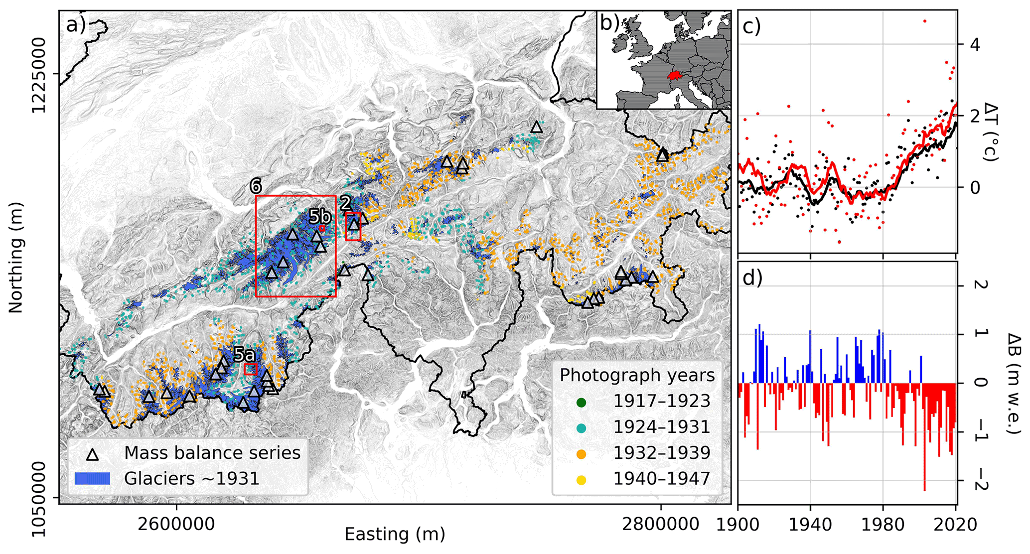
Figure 1(a) The distribution of Swiss glaciers around 1931 (blue areas). Country borders are outlined in black. The locations of the TerrA photographs used in the study are shown with coloured dots, whose colour indicates the year of acquisition. The red boxes show the bounds of other figures (figure numbers given in white). (b) The location of Switzerland (marked in red) in Europe. (c) Anomalies of mean annual (black) and mean summer (red) air temperature from 1961–1990; 10-year running averages are drawn as lines, and the data are from 14 homogenised stations (MeteoSwiss, 2021). (d) Mean anomalies in annual glacier mass balance compared to 1961–1990. The data are described in Sect. 2.3. Map coordinates are in the Swiss CH1903+/LV95 (EPSG:2056) coordinate system.
While topographic maps resolving Swiss glaciers have been drawn by the Swiss Federal Office of Topography (swisstopo) since the late 19th century, today's picture of glacier changes during the last century is largely based on a combination of (i) long-term glacier mass balance series extending back to the 1910s (GLAMOS, 1881–2020), (ii) repeated aerial photogrammetry acquired after the 1960s (Bauder et al., 2007), and (iii) model-based reconstructions (e.g. Huss et al., 2008). Such combined reconstructions are available for selected glaciers, and the results have been extrapolated to the regional scale (e.g. Huss, 2012). In this context, it is important to note that since the uncertainties in glaciological mass balance series are cumulative, they can cause large biases if not corrected with geodetic estimates over longer periods (Cox and March, 2004; Thibert et al., 2008; Zemp et al., 2010, 2013). For Swiss glaciers, such corrections have generally been based on mass changes derived from topographic maps before 1960 and later on from detailed geodetic surveys based on aerial imagery. However, uncertainties in the former datasets are large and sometimes difficult to quantify, especially for the first half of the 20th century. Modern reanalysis of the source material for these early maps, thus, holds great potential for further constraining the magnitude and lowering the uncertainty in estimates for past glacier changes.
From the First World War to the late 1940s, large parts of the Swiss Alps were surveyed by means of terrestrial (i.e. ground-based) photogrammetry. Engineers of swisstopo took photographs from about 7000 locations distributed across the country and measured both the terrain and the camera position with a phototheodolite (an angle-measuring device combined with a measuring camera). These surveys, which produced images that are now stored in what is known as the TerrA image archive (see Sect. 2.2), served as the basis for the production of the first national topographic maps with a scale of 1:50 000, as well as a set of military maps at the scale 1:10 000.
Here, we digitally process 21 703 terrestrial photographs acquired during the TerrA surveys by using modern photogrammetric methods and generate digital elevation models (DEMs) of nearly all glaciers in Switzerland (89 % by count). The images and DEMs refer to the time span between 1916 and 1947 (with a median year of 1931) and are used to reconstruct the geodetic glacier mass balance from 1931 to 2016 (Fig. 1). This is one of the rare regional reconstructions based on digital photogrammetry before the 1950s (e.g. Belart et al., 2020; Geyman et al., 2022) and, to the knowledge of the authors, the first of such scope to use terrestrial photographs as the source material.
2.1 Study site
According to the latest Swiss Glacier Inventory (SGI2016; Linsbauer et al., 2021), Switzerland presently contains ca. 1400 glaciers covering 961.4 ± 22 km2 in total. By area, this is about half of all glaciers in the European Alps (Paul et al., 2020). The Swiss glaciers currently span an elevation range between 1357 and 4599 m a.s.l., with a median elevation of 2913 m a.s.l. and a mean slope of 28∘ (Linsbauer et al., 2021). Both the median elevation and the mean slope are higher than the global average, which are 1308 m a.s.l. and 11∘, respectively (RGI Consortium, 2017). This relative steepness makes Swiss glaciers particularly suited for reconstructions based on terrestrial photogrammetry, as the steepness allows for favourable incidence angles of the photographs. In this study, we consider all glaciers on Swiss territory as long as suitable photographic material is available from the historical surveys (see below).
2.2 The TerrA terrestrial image archive
The TerrA archive consists of 57 385 images in total, covering most of the mountains in Switzerland, and the images were acquired during the first half of the 20th century. According to the images' approximate viewsheds (produced by swisstopo and distributed together with the images), about 21 703 (38 %) of these images cover glaciers.
Images were acquired from high points surrounding the surveyed areas (e.g. summits, ridges, slopes), and stereo acquisition was performed by taking two sets of pictures from locations spaced a few hundred metres apart (Fig. 2a). From each location, a panorama of about four to five images (Fig. 2b) was acquired to increase the viewing angle, with all images being acquired in the same orientation as their stereo-counterparts. About 86 % of the glacierised area is covered by at least two historical images from different physical locations, thus setting a constraint to the maximum theoretical coverage of the dataset. The actual coverage is lower as the incidence angle (i.e. the difference between the angle of the image and the terrain slope) is often low due to the photographs being acquired from the ground. This makes it difficult for feature-matching algorithms to obtain accurate results, thus lowering the coverage.
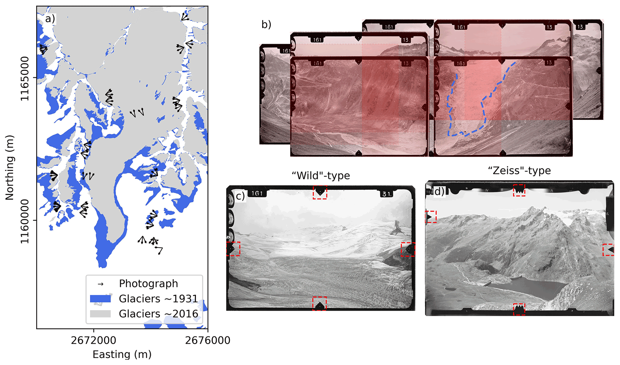
Figure 2(a) Imaging locations (black arrows pointing in the imaging direction) together with ca. 1931 (blue) and ca. 2016 (grey) glacier outlines for Rhonegletscher (alternatively Rhône Glacier). (b) Panorama example overlooking Rhonegletscher (outlined in dashed blue). The transparent red boxes show the coverage of each image. The darkest red indicates five images overlapping. (c, d) Examples of a “Wild”-type (c) and a “Zeiss”-type (d) photograph and associated fiducial marks (framed in red).
The 13 cm × 18 cm terrestrial images contained in the TerrA archive are scanned by swisstopo at a resolution of 21 µm, yielding digital images of 53 Mpx. The metadata of each image include an identifier for which stereo pair they belong to, the acquisition date, the position, and the viewing direction of the image as determined from field measurements. The photographs used in this study were acquired with 21 individual cameras between 1916 and 1947. Most photographs were acquired in the 1920s and 1930s, with a median year of 1931 and a standard deviation of 5 years. The cameras were of two different brands called Wild and Zeiss, which had different focal lengths, image dimensions, and frame geometry (Fig. 2c, d).
Within the 2008 “Action Plan for the Preservation of the Spatially Relevant Cultural Heritage of swisstopo”, it was decided to preserve the images in the TerrA archive, to scan them all, and to make them available to the public (Ryf and Klöti, 2008; Rickenbacher, 2012). After conceptual preparations, swisstopo started the project in 2013 and announced the release of the dataset in 2018 (swisstopo, 2018). To our knowledge, no scientific publication has used this unique digital dataset to date. The novel use of the imagery proposed here might thus pave the way for further utilisation of the archive.
2.3 Auxiliary data
Our processing workflow (see Sect. 3) requires a modern DEM as a reference for co-registration, as means of validation, and for calculating surface elevation changes with respect to the DEMs generated from the TerrA archive. We use the SwissALTI3D DEM (swisstopo, 2019) for this. This DEM is a 2 m × 2 m mosaic of lidar (below 2000 m a.s.l.) and digital aerial photography. Over glaciers, acquisition years range from 2007 to 2018, with a median year of 2016. The reported absolute accuracy of the DEM is between 0.1 and 3 m, depending on the location.
To exclude areas of possible elevation change over the 85-year period, we mask glaciers, perennial snowfields, and lakes. To do so, we use (i) the glacier and snow mask that Freudiger et al. (2018) digitised from the “Siegfried maps” made in 1917–1944 and (ii) the swissTLM3D product to mask natural and artificially dammed lakes (swisstopo, 2020).
The TerrA images were previously used to create the first edition of 1:50 000 topographic maps (the so-called “LK50”) in the alpine regions of Switzerland (swisstopo, personal communication, 2021). We use georeferenced scans of these maps to derive glacier outlines for all glaciers, which are proven here to be concurrent with the TerrA dataset. To digitise glacier outlines from the LK50 map series (see Sect. 3.1.3 for details), we use glacier outlines from the Swiss Glacier Inventory 1973 (SGI1973; Müller et al., 1976) as a template and follow the same naming convention for glacier identification. The SGI1973 is based on orthophotographs acquired in 1973 and represents the first accurate and complete mapping of Swiss glaciers.
Glacier outlines corresponding to the SwissALTI3D DEM are taken from the SGI2016 (Linsbauer et al., 2021). These are based on detailed mapping performed on orthophotographs with 0.1 to 0.25 m resolution and acquired during the period 2013–2018 (centre year 2016).
Different types of glacier mass balance data covering large parts of the study period are available from long-term monitoring efforts (GLAMOS, 2021). In particular, we use (1) time series of annual glacier-wide mass balance based on in situ observations, available for about two dozen glaciers and partly extending back to the first half of the 20th century (Huss et al., 2015, 2021); (2) geodetic mass balances computed by differencing up to 12 DEMs, in turn derived from either topographical maps or aerial photogrammetry (before and after the 1960s, respectively), available for about 50 glaciers at intervals between 3 and 60 years (Bauder et al., 2007; GLAMOS, 2021); (3) modelled time series of annual mass balances covering the period 1900–2021, obtained by updating the results from Huss et al. (2008, 2010a, c), who constrained a distributed daily mass balance model to match the observed glacier mass changes given by (1) and (2); and (4) country-wide, region-specific annual mass balances variations covering the last century, obtained by spatial extrapolation of the observations from (1) and (2) and supported by the modelling of (3) for the period before 1955 (GLAMOS, 2018).
The above data are used for both temporal standardisation of the heterogeneous imaging period and independent validation of the results (see Methods).
In this study, we process 21 703 images semi-autonomously to generate DEMs and measure glacier elevation change between 1931 and 2016. The main steps of the methodology are synthesised in Fig. 3, with detailed descriptions provided in the following subsections. In summary, images are preprocessed first to remove the geometric distortions introduced during digitisation (scanning) and to correct for biased position data (Sect. 3.1). Then, DEMs are generated for each stereo-panorama and co-registered to the modern stable terrain (Sect. 3.2). In a third step, the thus-derived DEMs are subtracted from the swissALTI3D DEM to obtain elevation change maps for the period 1931–2016. Temporal standardisation is performed to adjust the elevation change rates to the said period (Sect. 3.2–3.3.2). Finally, the glacier outlines derived from the digitisation of the LK50 map are used to mask the results and to obtain average elevation change rates and geodetic mass balances (Sect. 3.4).

Figure 3Flowchart synthesising the data processing. Inputs refer to the external data that were used; processes are different steps in the processing chain; outputs are files of particular interest for this study and future studies. All intermediate and output files are available for further use.
3.1 Image and data preprocessing
3.1.1 Fiducial mark detection
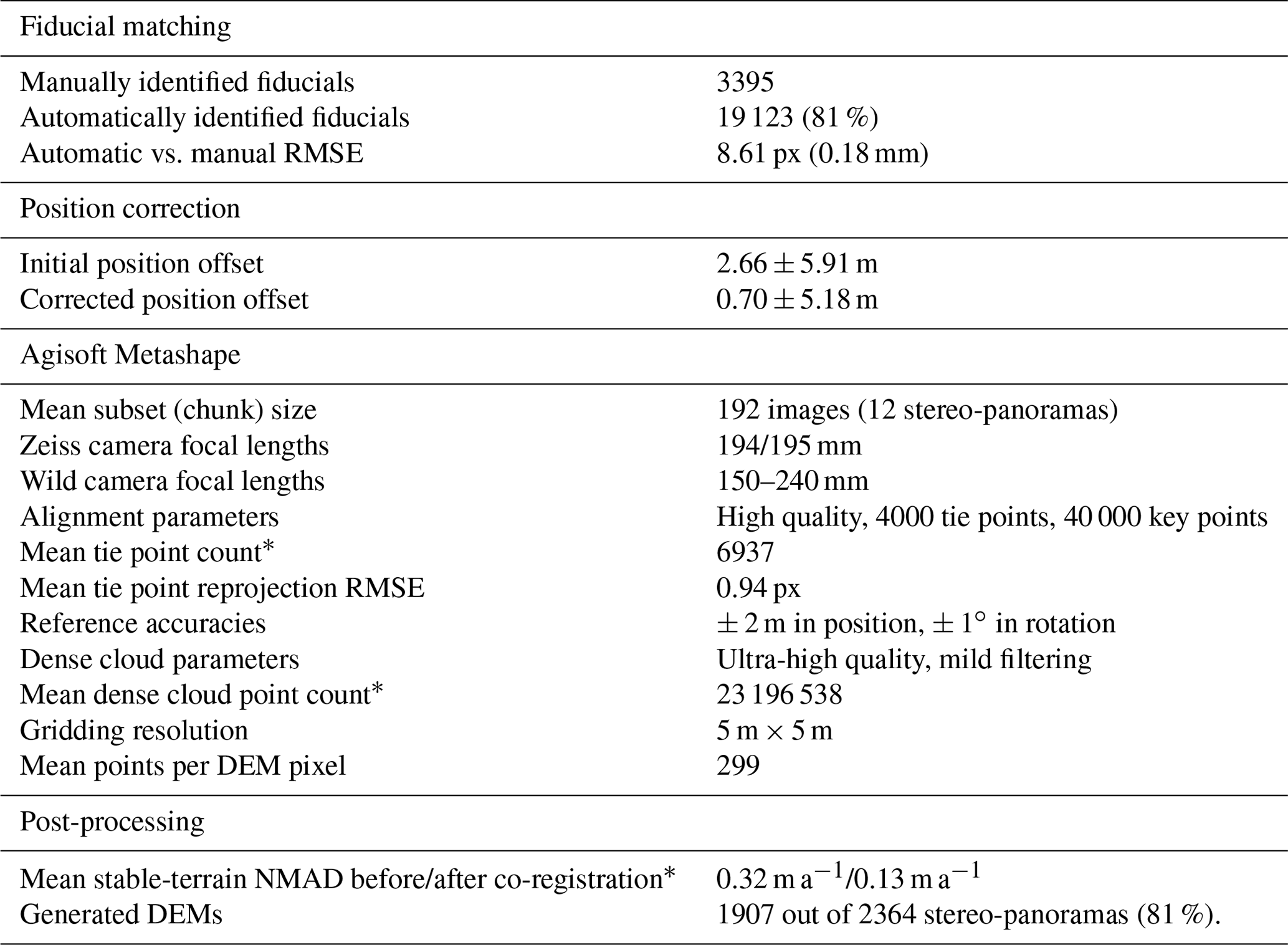
We use fiducial marks (small markers on the image frame as fixed references; red squares in Fig. 2c and d) to constrain the centre point and internal orientation of the imagery. The positions of the fiducial marks are used to calculate a transformation between the pixel coordinates and physical image coordinates. Undesired translations, rotations, or scaling effects introduced during scanning are removed though a similarity transformation estimated using the Python package “scikit-image” (van der Walt et al., 2014). Each image has four or more fiducial marks along its edges, with a size of about 350 px (∼ 7 mm). A theoretical minimum of two fiducial marks need to be identified, but more fiducial marks introduce redundancy and allow for exclusion of uncertain fiducial marks. We use a semi-automatic model to identify fiducial marks in the 21 703 images processed in the study. To calibrate the model, we manually identify fiducial marks in 3395 images (∼ 162 images per camera). Such a large calibration set was required because the 21 unique cameras in the dataset had slightly or completely different fiducial marks. We then use the manually identified fiducial marks to calibrate the model to do the same on the remaining 81 % of the image archive. Using template matching to identify the fiducial marks, the model estimates a similarity transformation and validates it using the residual differences between the identified fiducial marks and the modelled ones. We use random sample consensus (RANSAC) to exclude fiducial marks with residuals of more than 10 px (0.21 mm). The model found four and three fiducials filtered as inliers in 56 % and 32 % of the images, respectively, with a median manual-to-automatic transform root-mean-square difference of 8.61 px (0.18 mm). Model mismatches are largely due to film scratches, damage, or poor contrast in the images and are easier to identify manually than to account for in a more complex model. Hence, we manually identify the remaining 12 % of the images (with fewer than three automatic fiducials) to complement the automatic matches. In seven images, only two fiducials could be identified manually, but they are still used in spite of their higher potential error.
The border of each image needs exclusion to not interfere with the automatic image alignment. We create image frame masks by calculating the median intensity of all images of a given instrument (after applying the geometric transformation) and then segment the median image frame using thresholding.
3.1.2 Image position correction
A preliminary analysis of the digitised image metadata revealed spatially correlated biases in the image positions provided by swisstopo. We observe this by calculating the elevation difference between the image position and the SwissALTI3D elevation on stable ground. While this difference is expected to be the height of the tripod (∼ 1.2 m; swisstopo, personal communication, 2021), the calculated differences has an absolute bias of 2.66 ± 5.91 (mean ± SD) after taking the tripod height into account and an average horizontal offset of 0.66 ± 4.49 m. A possible explanation for these biases is that camera positions were estimated by triangulation from reference points, which in turn were all positioned relatively to other reference points. Therefore a small positional error could accumulate as the point is further away from the main reference. By sampling slope, aspect, and elevation values from the reference DEM at every recorded image position, we estimate the approximate 3D offsets from the image position data to the ground. We then partially correct the systematic component of the biases by averaging them in 1 km × 1 km grids and subtract the gridded offsets from the 3D positions of the images. This correction reduces the average difference between the DEM and the imaging locations to 0.70 ± 5.18 m (0.39 ± 4.15 m horizontally).
3.1.3 LK50 map series glacier outline digitisation
We obtain glacier outlines that are concurrent with the TerrA dataset by digitising outlines on the scanned and georeferenced LK50 map series (in the Swiss CH1903+/LV95 coordinate system; EPSG:2056) provided by swisstopo. Digitising glacier outlines from orthoimages generated in this study was also a theoretical possibility, but sporadic image coverage and time constraints led to the search for more efficient approaches. These orthoimages are thus only used to draw outlines for 61 sites, which are in turn used to validate the glacier outlines obtained from the LK50 series (see Sect. 3.5.2). The LK50 maps, made in the 1950s, cover all of Switzerland and are based on the TerrA photographs among other data. We manually digitise the glacier outlines of the LK50 maps by modifying the 2491 outlines (with a mean area of 0.60 km2) of the Swiss Glacier Inventory 1973 to fit the LK50 map data. This allows for the SGI1973 metadata to be easily retained and ensures consistency when including or excluding perennial snowfields as well as when drawing ice divides. We acknowledge that in this way, there is a potential underestimation of the change in the accumulation areas. Indeed, the outlines are only modified where they deviate from the SGI1973 outlines, meaning that minor deviations may be missed. We assume these potential discrepancies to be accounted for in our uncertainty analysis (Sect. 3.5.2). To reduce subjective error, outlines are drawn by one person and validation is performed by another.
3.2 Photogrammetry and DEM generation
We process the 21 703 images photogrammetrically in Agisoft Metashape version 1.6.5 in separate subsets (Table 1). Each subset consists of every image acquired with a specific camera over a single year, totalling 113 subsets, with 192 images each on average. We compute a separate camera model for each subset because of varying distortion parameters for each camera, depending on their construction and in which year they were used; differences may relate to the photographer, potential damage, and subsequent repairs the camera might have endured during its lifetime.
Table 1Photogrammetric processing parameters. The “high” alignment quality and “ultra-high” dense cloud quality mean using the full image resolution for each respective step. “Mild” (one-third strength) dense cloud filtering is a proprietary Metashape filtering setting. “NMAD” is the normalised median absolute deviation.
* Calculated values are averages for each individual stereo-panorama.
Within each subset, we align the stereo-panoramas individually using separate camera models. The ones that successfully align are then merged with a recomputed camera model. The discrepancy between camera models of different years is low for the estimated focal length (0.39 % standard deviation on average), while all other distortion parameters (radial, decentring, principal point offset, affinity, and skew) have a spread of 37 % on average. The large spread of the distortion parameters could indicate overfitting, but with acceptable tie point residual errors (Table 1), we choose to neglect this issue. The stereo-panoramas generally overlap with other panoramas in terms of detailed terrain, but the angle difference between extracted features is too large for the built-in feature matcher in Metashape to produce reliable tie points between stereo-panoramas. We therefore perform an alignment between all separate overlapping stereo-panoramas within a subset using iterative closest point (ICP) co-registration of dense point clouds that are constructed from each stereo-panorama. We use the ICP algorithm implemented in the Python package xDEM (version 0.0.5; xdem contributors, 2021), using core functionality from the OpenCV suite (OpenCV contributors, 2021). We run the co-registration in all areas where the dense clouds overlap, plus a buffer of ±15 m (chosen qualitatively through trial and error), to limit the co-registration to reasonable offsets.
Once the stereo-panoramas are aligned to each other, a new camera model is calculated with a bundle adjustment and new dense clouds are generated for each subset individually. We filter the dense clouds by excluding points with a “confidence” of less than or equal to 2. This threshold is chosen qualitatively by visually assessing the effect on noise for a few arbitrarily selected dense clouds. The confidence is a statistic provided by the Metashape software, but information on how it is calculated is unavailable. After the DEMs are generated from the resultant dense clouds and after orthoimages are generated using the DEMs, we co-register the DEMs to the SwissALTI3D DEM (Fig. 4a and b). This is done using the same ICP co-registration method as in the previous step but with the modern DEM as a reference outside of the unstable-terrain mask. We use the ICP transformation to correct the positional and rotational errors of both the historical DEMs and orthoimages. Finally, elevation change maps are generated by subtracting the DEMs from the reference SwissALTI3D DEM.
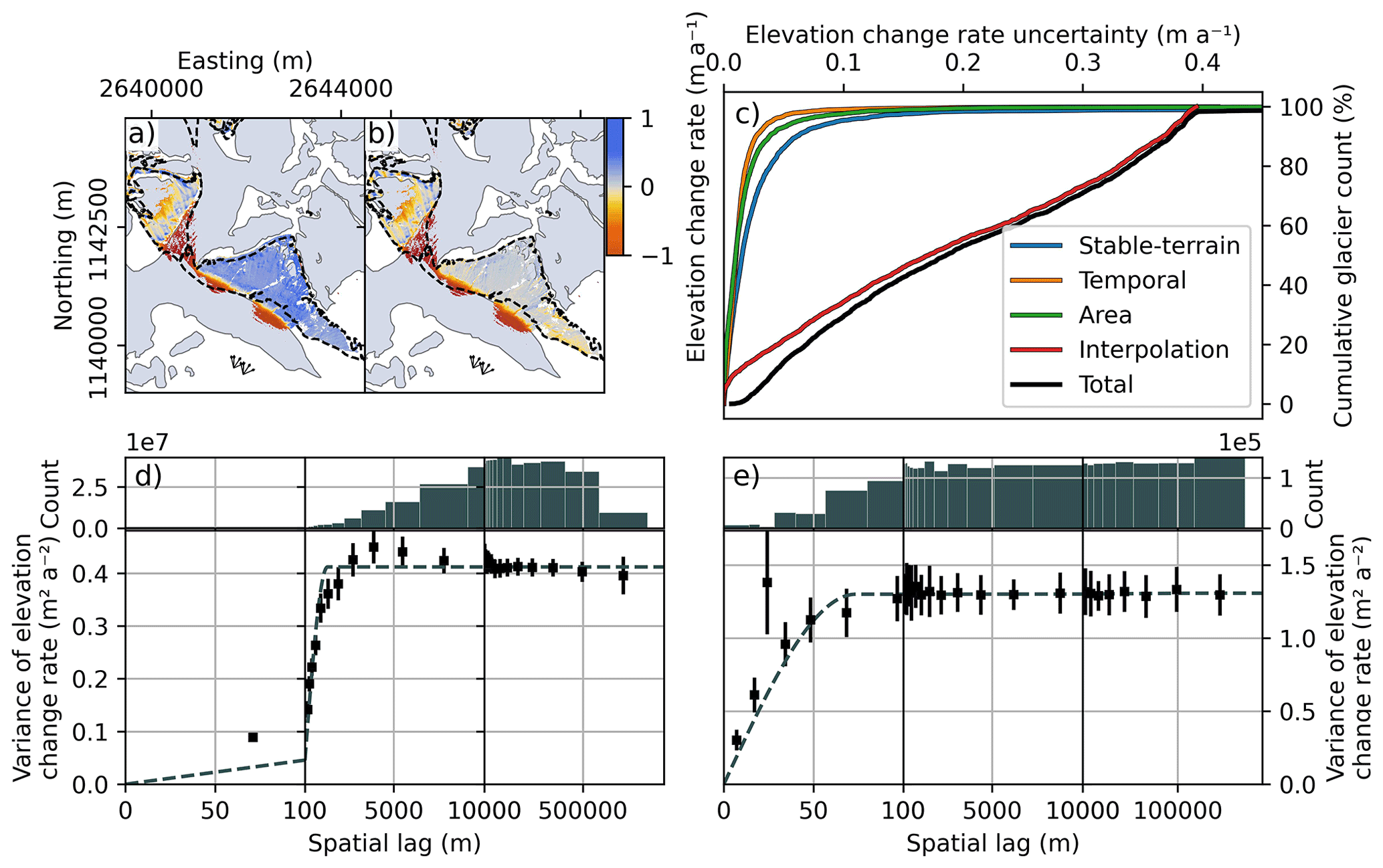
Figure 4Error figure ensemble. (a, b) Individual DEM difference before (a) and after (b) co-registration. The arrows indicate the locations and directions of the images used for generating the ca. 1931 DEM. The dashed lines indicate the theoretical viewshed of the stereo pair (pre-calculated by swisstopo). (c) Cumulative histograms showing the magnitude of the different components for the elevation change uncertainty of each individual glacier. (d, e) Variograms of interpolated (d) and stable-terrain (e) elevation difference uncertainties, showing the variance of all pairs of pixels at a given distance (or lag) as a function of that lag. The individual markers show the empirically derived variance; their error bars show their 95 % confidence intervals; the dashed line shows the variogram model (sum of two spherical models). The histograms above the variograms show the pairwise sample count for each empirically derived variance marker.
3.3 Post-photogrammetric processing
3.3.1 Temporal standardisation
Because both the historical and modern elevation datasets were acquired over several years (1916–1947 and 2007–2018, respectively), it is necessary to standardise the periods of observation for the evaluation and interpretation of the results.
We adjust each elevation change map to the median years 1931 and 2016 based on an annual dataset of observed mass balance variations that is specified for the major hydrological basins of the Swiss Alps (point 4 in Sect. 2.3). Regional anomalies in mass balance from the reference period 1961–1990 have been derived by spatially extrapolating all available series acquired using the direct glaciological method (between 8 and 20 glaciers; Huss et al., 2015; GLAMOS, 1881–2020). Before 1955, modelled mass balance variations for four glaciers were used (Huss et al., 2008). For each pixel, we calculate the ratio between the cumulative mass balance of the reference period 1931–2016 and the cumulative mass balance over the actual period of observation (Eq. 1). The elevation change rates over glacierised areas are then multiplied by this ratio to obtain the temporally standardised elevation change rate :
where t0 and t1 are the years of acquisition of the TerrA photograph and the SwissALTI3D DEM, respectively, and B(t) is the representative cumulative mass balance at year t for the given region.
3.3.2 Mosaicking and interpolation
We successfully generate 1907 elevation change maps, which we mosaic by averaging the temporally standardised elevation changes estimated at each pixel in a 5 m × 5 m grid. We exclude 3 out of the 1907 elevation change maps from the mosaic due to extreme median values ( m or >100 m). Regionally, 55 % of the total glacier area is missing from the elevation change mosaic due to incomplete image coverage and processing shortcomings, so an interpolation approach is required (Fig. 6). Gaps are spread over glacier extents throughout their elevation ranges, and we therefore chose to harness hypsometric interpolation approaches.
We use a modified version of the regional hypsometric approach (referred to as “global” in McNabb et al., 2019) where each glacier elevation change is normalised to its elevation range, i.e. scaling both elevation and elevation change from 0 to 1 for each glacier in 5th percentiles (Huss et al., 2010b). More specifically, we use the approach as implemented in the Python package xDEM. This approach relies on elevation changes estimated at different elevation bins and aims at capturing the glacier-wide hypsometric signal. Consequently, the quality of the interpolation deteriorates with decreasing spatial coverage. For our application, we choose this approach where >20 % of the glacier area is covered (91.1 % of all glaciers by area meet this criterion). For glaciers that do not meet this condition, we apply a simple regional hypsometric approach, in which gaps are replaced by the mean regional value within the same elevation band.
3.4 Glacier-specific and regional elevation change
We estimate glacier-specific elevation changes and geodetic mass balances for each SGI2016 outline individually. Then, we aggregate glacier-specific estimates to obtain regional-scale estimates.
For each individual glacier, we estimate the mean elevation change by averaging both the observed and the interpolated elevation changes that fall within the historical glacier outline:
Here, is the elevation change rate of a given pixel p and Np is the number of pixels within the glacier outline.
We then estimate the mean volume change rate by
where A0 is the glacier area as given by the historical glacier outline (referring to ca. 1931).
By applying a volume-to-mass conversion factor of ρΔV=850 kg m−3 (Huss, 2013), we estimate the glacier-wide specific mass balance rate using
where A1 is the glacier area as given by the SGI2016.
Similarly, we estimate the total glacier mass change rate from the volume change and the volume-to-mass conversion factor:
3.5 Uncertainty analysis
We identify multiple sources of error that propagate to our estimates of glacier volume and mass change. These sources include stochastic elevation change measurement errors, correlated short- and long-range DEM distortions, error in glacier outlines, the temporal standardisation, hypsometric interpolation, and the volume-to-mass conversion. We consider these sources separately and combine them into estimates of uncertainty for elevation, volume, and mass change. Throughout the text, uncertainties are within a 95 % confidence interval.
To propagate uncertainties from the pixel scale to the glacier scale and from the glacier scale to the regional scale, we estimate the spatial ranges at which errors are correlated. Where relevant, we perform this propagation by estimating the standard error with a number of effective samples (Neff) that account for spatial correlations. We derive the number of effective samples by numerically integrating a sum of variogram models fitted to our empirical variograms within a circular area of the same size as the glacier (Fig. 4; Hugonnet et al., 2021). This is a generalisation of the approach by Rolstad et al. (2009). We use the implementation in the Python package xDEM based on spatial statistics of the Python package SciKit-GStat (Mälicke, 2022).
3.5.1 Mean elevation change uncertainty
Multiple intermediate steps in the photogrammetric pipeline can distort DEMs and orthoimages. These include image scanning artefacts, camera model uncertainties, image noise, image location, and orientation error, as well as subsequent methodological shortcomings (Dehecq et al., 2020). We quantify the uncertainty comprising these errors by comparing terrain assumed to be stable in our elevation change estimates. Stable terrain excludes ice, perennial snow patches (Freudiger et al., 2018), and lakes. Dams created between the 1920s and 1980s are especially important to exclude as they otherwise introduce unwanted positive changes of up to >50 m. While other factors such as landslides, vegetation change, and buildings may also affect stable terrain, visual inspection showed no obvious signs of their presence.
For DEMs generated by satellite or airborne photogrammetry, elevation change errors often vary with terrain aspect, slope, or curvature (Toutin, 2002; Hugonnet et al., 2021). Here, we find no dependency of the uncertainty in elevation change on these terrain attributes. We suspect that this is the result of the large number of DEMs that is used in our mosaic. Indeed, DEMs derived from terrestrial images might be affected by such attribute-dependent errors, but since the individual DEM tiles are derived independently from an independent set of images, these should cancel out when aggregated over several glaciers. We thus assume that our elevation uncertainty is stationary in space and estimate it by using the normalised median absolute deviation (NMAD) of the elevation change estimates on stable terrain.
We account for spatial correlation of elevation change uncertainty by fitting a double spherical variogram model to the empirical variogram of elevation changes (Fig. 4d and e), thereby modelling short- and long-range correlations (in stable-terrain residuals, panel e, and interpolation errors, panel d). We then estimate the uncertainty in the mean elevation change rate σ by circular integration of the sum of variogram models over the glacier area A (Rolstad et al., 2009; Hugonnet et al., 2021):
where σp is the NMAD of elevation differences on stable terrain, γ(l) is the sum of variogram models with spatial lag l, and Neff is the number of effective samples.
3.5.2 Glacier outline uncertainty
We identify three major sources of uncertainties from the glacier outlines drawn from the LK50 maps: the georeferencing error of the map, the timing uncertainty of the topographic data used (which is unknown but was assumed to largely be the TerrA dataset), and the errors in manual delineation (including the subsequent digitisation from the map) of a glacier front. The temporal concurrency of the LK50 map with the TerrA imagery particularly needs validation as the extent to which data from other times were used is unknown. In the case where the outlines are spatially consistent with the TerrA dataset, the concurrency assumption is verified.
We evaluate these three uncertainty sources combined by digitising sparse outlines at 61 sites from orthorectified versions of the photographs generated in the photogrammetric pipeline. We then compare their general agreement with the LK50 glacier outlines. Outlines drawn from orthoimages will have a perfect relative georeferencing to the DEMs and should thus only differ from the LK50 outlines due to the subjective nature of glacier delineation. For this comparison, we draw lines from the centroid of each glacier toward arbitrary points on the digitised outline and measure the distance to each LK50 and orthoimage-derived outline intersection. We use the difference between the two as a metric of the variability in spatial extent (Fig. 5b).
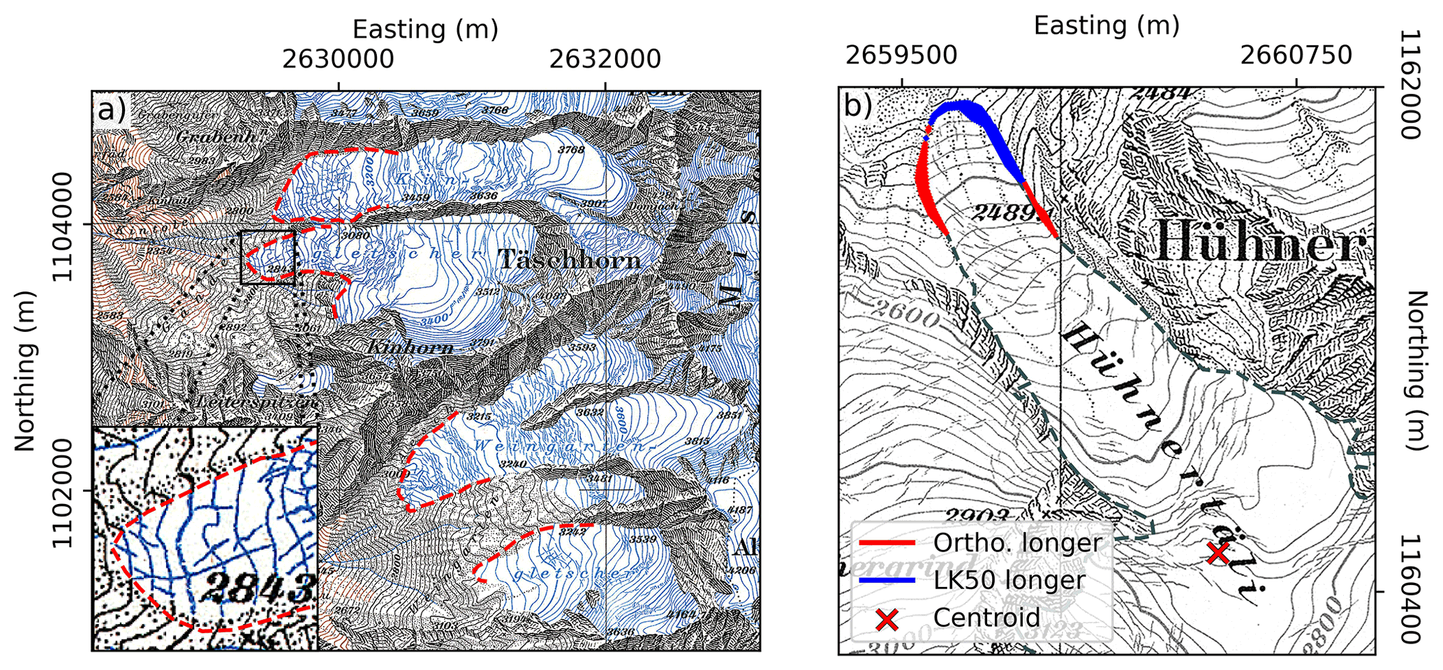
Figure 5(a) Glacier outlines drawn from orthoimages generated in this study (dashed red), superimposed on a sheet of the LK50 map series. (b) Comparison between glacier outlines derived by digitising the LK50 map series and orthoimages. Red shading indicates that the outline drawn from the orthoimage is farther away from the centroid than the outlines derived from the LK50 map series. Blue shading indicates that they are closer.
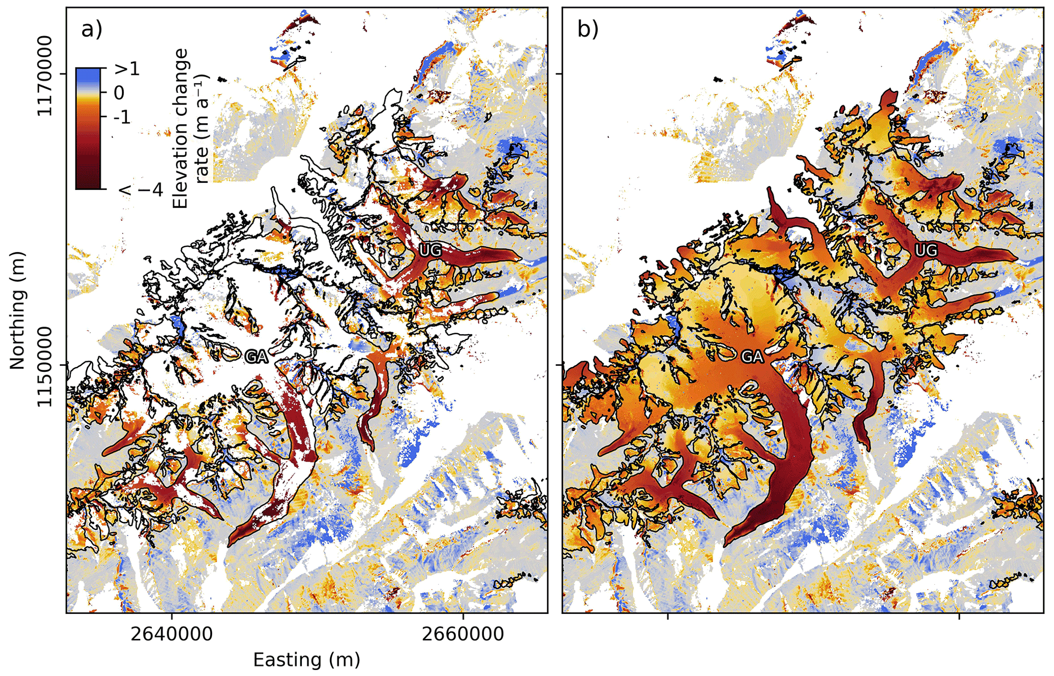
Figure 6Maps of average ice thickness change rates (dH dt−1) over the period 1931–2016 before (a) and after (b) interpolation. The area shows Grosser Aletschgletscher (GA; alternatively Great Aletsch Glacier), Unteraargletscher (UG), and other neighbouring glaciers. Glacier outlines from ca. 1931 are drawn in black.
We find a resultant median length difference of 7.9 m; the LK50 outlines are generally less extensive, possibly due to manual delineation differences in including or excluding glacier-marginal snow cover, with an NMAD of 28.06 m. Finally, in order to propagate these delineation differences into a source of elevation change uncertainties, we first dilate (i.e. enlarge) and erode (i.e. shrink) the mask by the systematic difference (7.9 m). We then estimate the glacier outline uncertainty by computing the average difference between the initial mask and the dilated or eroded masks:
where is the mean elevation change rate within the dilated mask and is the mean elevation change rate within the eroded mask.
3.5.3 Interpolation uncertainty
We estimate the uncertainty in the interpolation approach by artificially introducing gaps into the gap-free elevation changes of Hugonnet et al. (2021). These elevation changes are based on stereo-correlation of optical satellite imagery from the Advanced Spaceborne Thermal Emission and Reflection Radiometer (ASTER), which covers the entire study area and refers to the period 2000–2020. We interpolate the introduced gaps using our approach and study the difference between the interpolated ASTER elevation changes and the original ASTER elevation change estimates. We use this difference solely to compute the spatial correlation of uncertainties. For this, we fit a double spherical variogram model to the empirical variogram of the above difference in elevation change. We thereby measure the spatial correlation range of the error in interpolated elevation changes (Fig. 4d). In order to scale the variance of our interpolation uncertainty σint correctly, we did not use the NMAD of ASTER differences, which have a different absolute magnitude and could be biased by a lesser vertical precision. Instead, we interpolate the TerrA elevation changes for all pixels and then use the NMAD of the difference between the original and interpolated elevation change estimates.
We find strong correlations of interpolated elevation change errors at pixel scales, which fully decorrelate at a spatial lag of approximately 2100 m. This indicates that errors are strongly correlated at the glacier scale but are largely independent between glaciers of a given region. We thus propagate our interpolation uncertainties from pixel to glacier or region using Eq. (6). We then add a 0.01 m a−1 1σ symmetrical uncertainty to conservatively account for the median bias found in the difference between the interpolated and original elevation changes from ASTER.
3.5.4 Temporal standardisation uncertainty
We perform our temporal standardisation using modelled mass balance estimates, whose uncertainties accumulate over time. The reported uncertainty for annual specific mass balance (σB) based on in situ glaciological observations is approximately 0.2 m w.e. a−1 (Zemp et al., 2013). We derive the uncertainty in the temporal standardisation by standard propagation of independent uncertainties:
where B(t) is the cumulative mass balance for year t and where the standardisation is carried out for the time period t0–t1.
3.5.5 Total elevation change uncertainty
We calculate the total glacier-specific and regional uncertainty in mass balance by the squared sums of all error components, accounting for the number of effective samples (Neff) derived from the variograms where appropriate:
Here, σtopo is the NMAD of the stable-terrain difference, Ntopo is the number of effective samples calculated from the stable-terrain variogram model (Fig. 4e) and using Eq. (6), σint is the NMAD of the difference between the artificially removed and interpolated pixels, Nint is the number of effective samples calculated from the interpolation error variogram model (Fig. 4d, Eq. 6), is the absolute average mass balance rate for the glacier or region, and kg m−3 is the uncertainty in the factor used for volume-to-mass conversions (Huss, 2013).
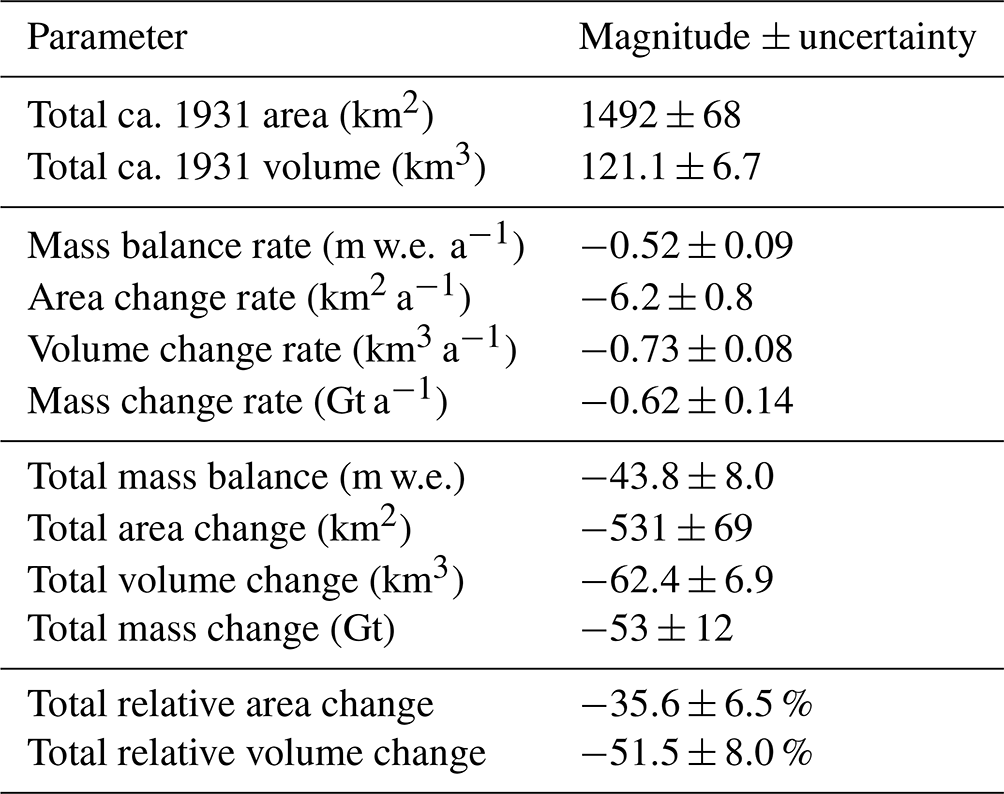
For the period 1931–2016, our results indicate an average glacier volume loss of 0.73 ± 0.08 km3 a−1 and a mean annual specific mass balance of −0.52 ± 0.09 m w.e. a−1 (Table 2). With a total Swiss glacier volume of 58.7 ± 2.5 km3 in 2016 (Grab et al., 2021), this corresponds to a loss of 0.86 ± 0.08 % per year compared to the 1931–2016 average volume. Integration of these changes over the considered period provides a total glacier volume loss of 51.5 ± 8.0 % since 1931 (0.15 ± 0.03 mm sea level equivalent assuming 361.8 Gt mm−1; Hugonnet et al., 2021). The total glacier area concomitantly reduced by 6.2 ± 0.8 km2 a−1, corresponding to an area loss of 35.6 ± 6.5 % (the total glacier area was 1492 ± 68 km2 in ca. 1931 and 961 ± 22 km2 in 2016).
Table 2Swiss-wide change rates and total changes in specific mass balance (B), thickness, area, volume, and mass from 1931–2016. See Eqs. (2)–(5) for how these are calculated. The uncertainties are the 95 % confidence intervals.
We analyse the spatial variability in mass balance over a regular grid of 30 km × 30 km (Fig. 7). The results show relatively high spatial variability, as shown by the ca. 1.5× larger mass loss rates in the Aletsch region compared to the southern Valais Alps. On the same grid, we observe a minimum regional loss of 0.32 m w.e. a−1 in the south-west and a maximum loss of 1.02 m w.e. a−1 in the north-east (only cells with more than five glaciers are considered).
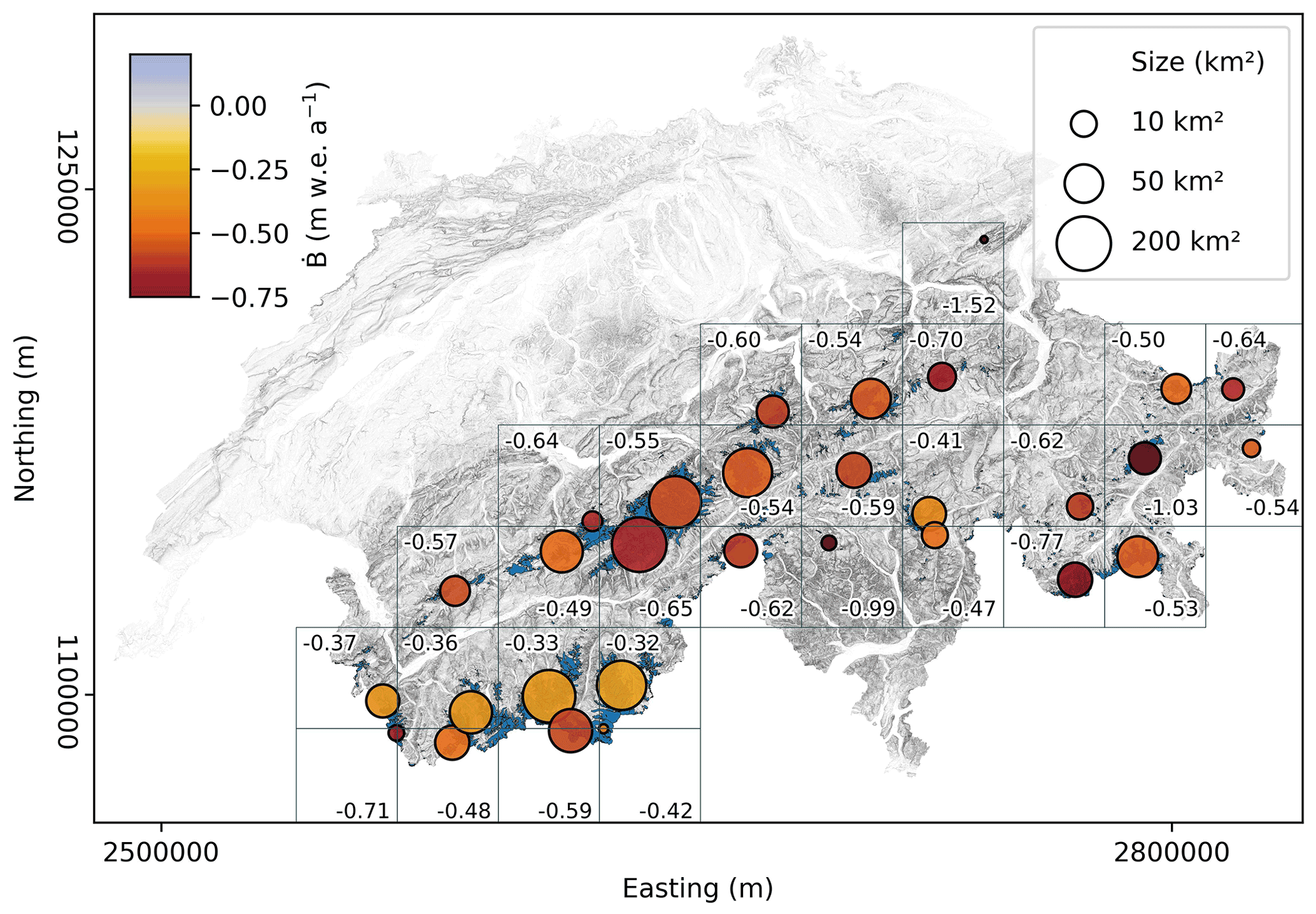
Figure 7Area-weighted geodetic mass balance rates (colours and numbers) for 30 km × 30 km tiles (grey squares). The location of each circle is the average glacier centroid weighted by area in the tile, and their sizes indicate the glacier area in ca. 1931.
Analysing the regional mass balance as a function of the easting and river basin (Fig. 8) reveals a clustered elevation dependency for individual basins. In general, glaciers in the central part of the Rhône basin have a higher median elevation and lower mass loss compared to other basins. We also observe a Pearson correlation coefficient of r=0.42 between the glacier mass balance and median elevation (Fig. 9a), indicating that lower glaciers appear to experience higher mass loss rates. From these two results, we can conclude that the regional variability in mass balance across the Swiss Alps is largely influenced by glaciers' median elevation.
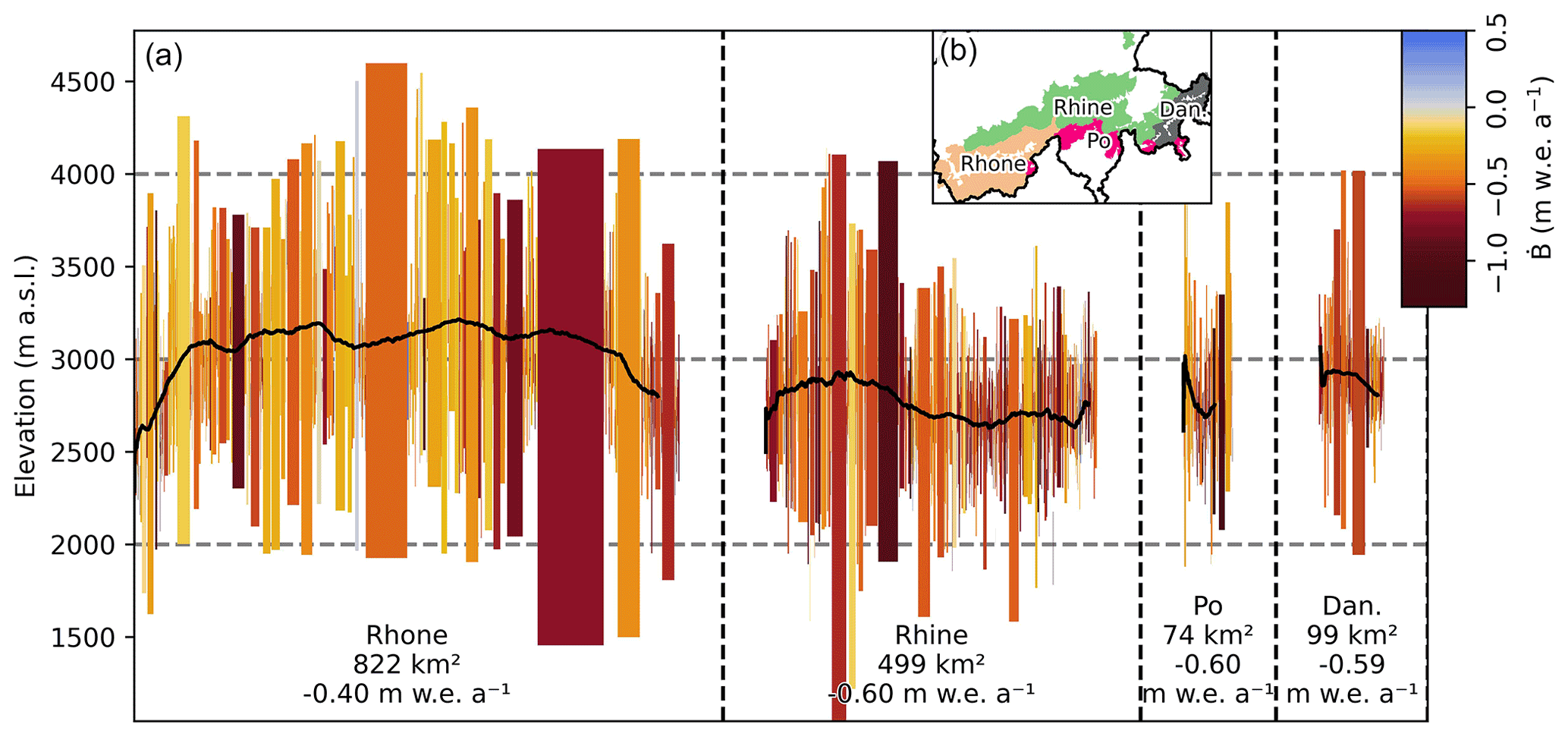
Figure 8West-to-east transect of glaciers in Switzerland (a), grouped by the four main drainage basins (b). Each bar represents a glacier; the width indicates the ca. 1931 glacier area; the colour shows the average geodetic mass balance from 1931–2016; the lower and upper bounds show the glacier's modern elevation range. The near-horizontal black lines are moving averages of the median glacier elevations. For each drainage basin, the total area as of ca. 1931 is given, together with the average geodetic mass balance weighted by glacier area.

Figure 9Area-weighted 10th percentile (0 %–10 %, 10 %–20 %, etc.) boxplots showing the relations between 1931–2016 average glacier mass change rates (vertical axes and colours) and different morphological parameters (horizontal axes). The whiskers extend from the box by 1.5× the inter-quartile range (IQR). The stated Pearson correlation coefficients (r) refer to the unbinned variables. (a) Correlation with median glacier elevation, indicating that lower elevations show larger mass loss rates. (b) Correlation with glacier area, showing no clear relation. (c) Correlation with the slope of the lowermost 10 % of the glacier surface, possibly showing higher mass change rates for glaciers with flatter termini. (d) Correlation with fractional debris cover in 2016 (taken from Linsbauer et al., 2021), indicating that higher mass change rates may be found for glaciers with high debris-coverage percentage.
Weaker correlations with other morpho-topographic characteristics are detected as well. For example, we observe a correlation between glacier mass balance and the mean slope of the lowest 10th percentile of elevation (r=0.28; “terminus slope”; Fig. 9c) and a similar negative relationship with modern fractional debris cover (; Fig. 9d). This indicates that glaciers with flatter termini or a higher debris-cover fraction tend to experience higher mass loss rates than their steeper and ice-free counterparts. These findings support the results from studies performed with smaller subsets of Swiss glaciers (Huss, 2012), over shorter time spans (Fischer et al., 2015), in different geographical regions (Brun et al., 2019; Geyman et al., 2022), or based on area change data (Linsbauer et al., 2021).
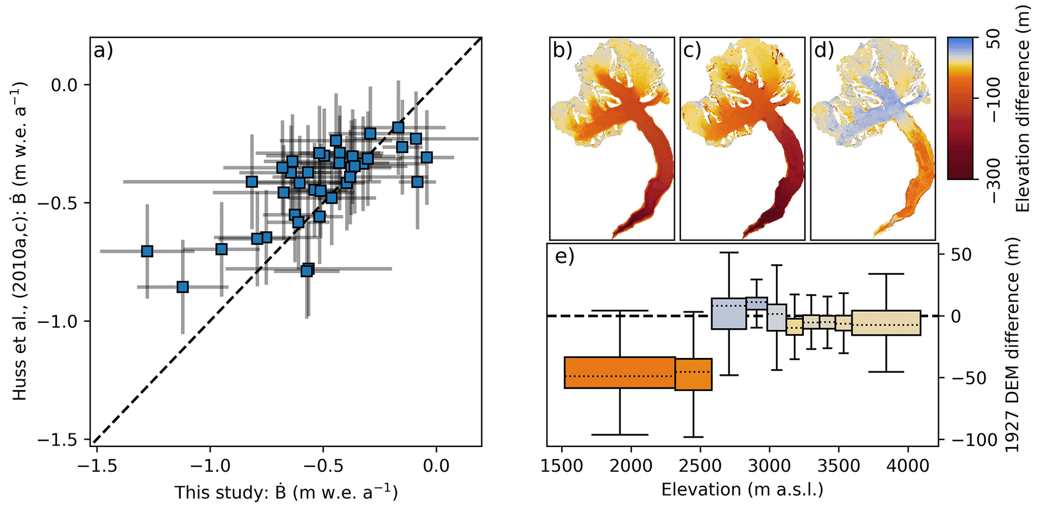
Figure 10(a) Comparisons in the same time-intervals of 39 glacier-wide mass balances inferred in this study with mass balance derived from modelling, constrained by geodetic surveys at decadal intervals (blue squares; Huss et al., 2010a, c). The Pearson correlation coefficient between the points is 0.71. The horizontal uncertainty bars are the 95 % confidence intervals of this study; the vertical uncertainties are fixed uncertainties of 0.2 m w.e. a−1 (see Sect. 5.1); the dashed line is a 1:1 line. (b) Elevation difference between the 1927 topographic map digitised and used by Bauder et al. (2007) and the SwissALTI3D DEM in 2017. (c) Elevation difference between the DEM mosaic generated in this study and the SwissALTI3D DEM in 2017. (d) Difference between the 1927 topographic map and the DEM mosaic from this study (map − this study). (e) Differences between the two 1927 DEMs (see d) binned for every 10th percentile of elevation. A general agreement is seen on the upper part of the glacier (above ∼ 2700 m a.s.l.), but the tongue is portrayed as smaller in the topographic map.
5.1 Comparison with previous glacier-wide estimates
The current consensus on the magnitude of Swiss glacier changes over the 20th century stems from (i) the work by Bauder et al. (2007), who derived glacier volume changes from the digitisation of topographic maps and the evaluation of repeated aerial photogrammetrical surveys for 19 large glaciers, and (ii) the combination of the analysis by Bauder et al. (2007) with direct glaciological measurements and modelling, extended to 39 glaciers (Huss et al., 2010a, c; GLAMOS, 1881–2020). Since the topographic maps relied on the TerrA surveys, comparing our results with these previous estimates is particularly relevant. We thus extract the cumulative mass balance for each of the 39 glaciers considered in previous studies and compare these results to our estimates (Fig. 10a). We find generally good agreement at the scale of the individual glaciers (r=0.71), although the results from the previous studies (Bauder et al., 2007; Huss et al., 2010a) indicate a mass loss rate that is, on average, 0.08 m w.e. a−1 smaller than ours.
For Grosser Aletschgletscher (location shown in Fig. 6), we additionally compare the map data digitised by Bauder et al. (2007) to the DEM mosaic we generated for 1926 and 1927 (Fig. 10b–e). The mean thickness change derived from the map is −56 m (with an unknown uncertainty), while the results of our study suggest a change of −72 ± 10 m (Fig. 10b and c, respectively). Comparing the two DEMs reveals an elevation-dependent difference (Fig. 10d–e): the results generally agree in the accumulation area but differ considerably at the low glacier elevations. We attribute this difference to (i) poor georeferencing of either dataset; (ii) temporal inconsistencies in the map data, which might not uniformly represent the year 1927; or (iii) a combination of these factors. Also note that for being consistent with Bauder et al. (2007), the above values are obtained by excluding the tributary Mittelaletschgletscher. Before 1969, the latter was confluent with Grosser Aletschgletscher (GLAMOS, 1881–2020; this is also reflected in the LK50 outlines). Similar outline inconsistencies at other glaciers might contribute in explaining differences between the two studies as highlighted in Fig. 10a.
The above comparison also reveals a potential shortcoming of our interpolation approach near the glacier margins. Indeed, the proximity to glacier margins was not considered, meaning that changes can be overestimated at these specific locations. The problem arises from the fact that our gap-filling procedure is based on the multiplication of the average ice thickness change rate observed at a given elevation with the length of the considered time period (i.e. 1931–2016, on average). This results in a total, elevation-dependent ice thickness change that is added back to the SwissALTI3D DEM. For a given location, however, the actual surface elevation in 1931 might have been smaller, especially if the location became ice-free before 2016. The latter case is most often encountered near the glacier margins, which explains the pattern of differences observed in Fig. 10d and e.
While the above shortcoming is inherently accounted for in our uncertainty analysis, we suggest that future studies could improve the interpolation technique used here. Auxiliary information on the timing at which a given location has become ice-free might help with that. Assuming that the uncertainty in the maps used by Bauder et al. (2007) is similar to or larger than in our study, however, the 95 % confidence intervals of the mean thickness change overlap.
5.2 Comparison with the regional estimate of Huss (2012)
To date, the only Swiss-wide estimate of glacier volume changes over a century is provided by Huss (2012), who extrapolated mass balance time series available for 50 glaciers by using a multi-parameter regression. The study refers to the period 1900–2011 and estimated a total volume loss of −42.1 km3, corresponding to a mean surface mass balance of −0.28 m w.e. a−1. To make these results comparable to our study, we updated the estimate to the period 1931–2016 by using the same methodology as in the study by Huss (2012). This results in a Swiss-wide volume loss of −44.8 km3, which is 28 % smaller than our estimate. The reasons behind this discrepancy might be twofold: for one, our interpolation scheme may overestimate thinning over retreating glacier areas (see Sect. 5.1) and, for another, the two studies are based on two different glacier inventories (we rely on the SGI2016, while Huss, 2012, relied on an inventory from 2003). Here below we discuss these two possible explanations in more detail.
To evaluate the influence of our interpolation scheme, we estimate the range of the associated bias in two ways. (1) In the first way, we simply assume a constant bias of −0.08 m w.e. a−1 for our estimate, i.e. 15 % of the total volume change (see Sect. 5.1). This results in a correction of +9.4 km3. Note, however, that such a correction implies the strong assumption that map-based observations are error-free, which seems difficult to defend. (2) In the second way, we consider that the interpolated thinning rates over now-deglacierised pixels could be overestimated by a factor of 2. This factor of 2 results from the assumption of a constant thinning rate and a constant glacier retreat. In such a case, indeed, the average thinning experienced by the area that deglacierised between 1931 and 2016 would be the average between zero (i.e. the thinning experienced by pixels at the glacier boundary in 1931) and the maximum thinning (i.e. the thinning experienced by pixels at the glacier boundary in 2016), while in our method all interpolated values are set to the maximum thinning (this is because the year at which a given pixel deglacierised is unknown). From the (i) deglacierised area (Table 2), (ii) average elevation change over deglacierised pixels with interpolation (−50.8 m), and (iii) fraction of deglacierised interpolated pixels (0.44), we estimate a correction of +5.8 km3. The two ways thus indicate that our interpolation scheme could introduce a negative bias of 5.8–9.4 km3. Since the exact bias is unknown, however, we prefer to provide the uncorrected estimates and to account for the bias in our uncertainty assessment.
In relation to the different glacier inventories used by Huss (2012) and by us, we note that many small glaciers have disappeared between 1931 and 2003 (i.e. the year of the inventory used by Huss, 2012). These glaciers could not be accounted for in the Huss (2012) estimate. To quantify this effect, we identify all disappeared glaciers, i.e. all glaciers polygons in the 1931 inventory that do not overlap with any polygons of the 2016 inventory. We find that such glaciers account for 68 km2 of the area loss and for 2.3 km3 of the volume loss since 1931. The latter corresponds to 3.6 % of the loss estimated for the whole sample. The mean thinning rate for these glaciers is roughly 25 % lower than the regional average, which can be explained by the fact that the thinning is bounded by the initial ice thickness. The contribution of 3.6 % from disappeared glaciers is slightly smaller but comparable to the 5 %–6 % contribution estimated by Parkes and Marzeion (2018) for glaciers at the worldwide scale.
When combining the above considerations, i.e. when applying a possible correction of between 9.4 and 5.8 km3 because of the interpolation method and when accounting for a 2.3 km3 difference because of disappeared glaciers, our estimated volume loss would come to lie in the range of 50.7–54.3 km3. This is still ca. 15 % larger than the estimate by Huss (2012) but reconciles the two estimates within their respective uncertainties.
5.3 Main drivers of variability in glacier mass loss
To better understand the drivers of glacier mass balance, we perform a multivariable regression analysis identical to that in Huss (2012). When doing so, we estimate the fraction of variance explained by each explanatory variable by calculating the difference in the coefficient of determination (R2) between the case in which the given variable is included and the case in which it is not. Table 3 shows that the highest portion of variance is explained by the median glacier elevation, followed by the glacier area. The glaciers' easting and northing, as well as the mean glacier aspect (tested for consistency with Huss, 2012), only explain a negligible fraction of the variance and are therefore excluded from further analysis.
Table 3The relative importance of each glacier variable in a multivariable regression to explain the variance of glacier mass balance (see Huss, 2012). The total R2 of the multivariable regression using all parameters is 0.46; the “New R2” column for each parameter is the explained variance when excluding the parameter in question, and the “R2 diff.” column is the difference in percent to the total R2. The coefficient sign shows if the parameter is positively or negatively correlated with glacier mass balance.
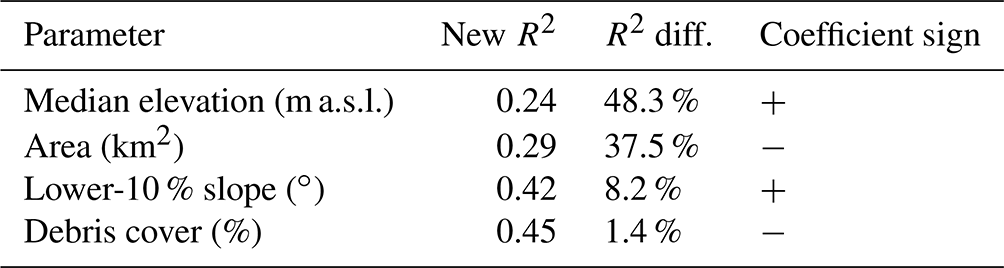
These findings are similar to the ones by Huss (2012), except for the fact that median elevation has a higher importance than glacier area in our study (Huss, 2012, found the opposite). The difference may be due to the different sample sizes (50 and 2491 glaciers, respectively), the different glacier outlines (which directly affect the glacier area), or the different time intervals. While the importance of the median elevation is clearly reflected in a direct correlation with the determined mass change rates (Fig. 9a), the importance of glacier area is more nuanced and only a weak correlation is observed (Fig. 9b). This could imply a co-variance between glacier area and another parameter (such as the median elevation), which, in combination, would help explain the observed variance in mass balance.
We attribute the correlation between median elevation and glacier mass loss to differences in regional snow accumulation: as the forcing resulting from air temperature is similar throughout the Swiss Alps (Isotta et al., 2019), we hypothesise that variations in median glacier elevation (Fig. 8) are driven by differences in precipitation totals that are reduced in the inner alpine regions of the Valais and Eastern Switzerland (GLAMOS, 1881–2020). A glacier located in a region with a drier – or more continental – climate will thus experience a higher median elevation. In turn, precipitation totals are known to determine altitudinal mass balance gradients, and hence the sensitivity of glacier mass balance to changes in air temperature (Oerlemans and Reichert, 2000; Rasmussen and Andreassen, 2005). In summary, regions with smaller precipitation are characterised by higher glacier median elevation and, hence, reduced climate change sensitivity, resulting in less negative mass balance compared to regions with high precipitation totals.
The single observation time period in our study (1931–2016) prevents us from analysing the climatic factors (e.g. temperature, precipitation) that control the temporal variability in glacier mass balance. Such an analysis was already performed by Huss et al. (2010a), who used annual mass balance series and found that the multi-decadal mass balance variability is significantly anticorrelated to the Atlantic Multi-decadal Oscillation. By leveraging different datasets, e.g. from repeated aerial surveys or satellite observations, it would be possible to obtain more frequent observations (Bauder et al., 2007; Rastner et al., 2016; Mölg et al., 2019). This could help constrain the multi-decadal variability in glacier mass changes but is understandably beyond the scope of our study.
5.4 Advantages and challenges of digital reanalysis
Reanalysis of the source material is a clear step forward compared to the map-based analyses that have been available so far (see Sect. 5.1). This is because the generation of topographic maps requires considerable interpretation and sometimes qualified guesswork to connect points of known elevation with continuous contour lines. The two factors make for a fuzzy border between actual data and subjective inter- or extrapolation. Comparisons between glacier extents obtained from digitised maps and modern digital photogrammetric reconstructions show significantly reduced biases for the latter (e.g. Koblet et al., 2010; Midgley and Tonkin, 2017; Geyman et al., 2022). In addition, many maps are temporally inconsistent. This is because maps are asynchronously updated with newer data, which are added to older maps during successive revisions. Problematic in this respect is the fact that, at least for Switzerland, the exact year of the data used during such revisions is mostly unknown (Fischer et al., 2015). This issue has been solved for maps referring to the second half of the 20th century, where precisely dated and complete surveys based on aerial photogrammetry have become available. This is an important step forward, especially for glaciers with long-term monitoring programmes (Bauder et al., 2007).
While the temporal consistency of our results is warranted in general, some uncertainty is introduced through the temporal standardisation required for individual glaciers. For individual glaciers, this uncertainty is generally below 0.09 m w.e. a−1 (see Sect. 3.3.1 and Fig. 4c). Such temporal inhomogeneity of country-wide results is inherent to any analysis that is based on terrestrial surveys. Indeed, the time required to acquire such data will always lead to a temporal spread in the time of acquisition. Although this problem is decreasing in importance for modern surveys thanks to a wider image swath, the analysis of historical photographs requires careful consideration of the issue. We suggest that temporal standardisation, in line with (or better than) our study, is a fundamental step in post-processing and interpreting the results derived from historical surveys – especially terrestrial ones.
Future improvements in our workflow may help further increase the spatial coverage of the dataset and reduce co-registration errors. While our Swiss-wide total specific mass balance uncertainty is low (0.09 m w.e. a−1), uncertainties at the scale of individual glaciers are on the same order of magnitude as (and sometimes higher than) the magnitude of the change (0.01–0.62 m w.e. a−1, with a median of 0.17 m w.e. a−1). The interpolation necessary over 55 % of the analysed area was the largest contributor of uncertainty in our analysis (0.00–0.39 m w.e. a−1 for individual glaciers; Fig. 4c). Higher coverage or a more accurate interpolation method may reduce this. The TerrA dataset has a theoretical maximum glacier coverage of ca. 86 %, meaning that only about half of the theoretical maximum was realised in our reconstruction. Newer photogrammetric methods, especially those rooted in the machine learning domain (e.g. Mildenhall et al., 2020; Zheng et al., 2020; Sarlin et al., 2020), can help improve feature description or depth reconstruction. This may increase the coverage of the resulting datasets compared to the methods currently implemented in Agisoft Metashape. In this respect, we attempted to replace the feature matcher with ASIFT (Morel and Yu, 2009), but long processing times and a general lack of robustness to image noise led us to abandon the idea.
Concerning the TerrA dataset, it is remarkable that reanalyses such as that presented here are possible at all for a dataset that is almost 100 years old and in some cases even older. This possibility is only provided by the systematic, thorough, and meticulous archiving that was performed at that time and by the preservation efforts that have been invested since then. The Swiss Federal Office of Topography deserves credit for this. In this context, it is interesting to note that what have now become known as the “FAIR Guiding Principles for scientific data” (Wilkinson et al., 2016) were respected over the course of almost a century. Indeed, the FAIR principles require the data to be findable (F), accessible (A), interoperable (I), and reusable (R), and all of these criteria are met for the TerrA archive: the images are easily found and accessed via swisstopo’s geodata portal (https://www.swisstopo.admin.ch/en/geodata/images/terrestrial.html, last access: 1 July 2022), are made interoperable by being distributed in a commonly accepted digital data format, and are reusable thanks to the rich and self-explaining metadata that complement the individual images. Similar databases exist in many other countries including, although not limited to, the United States of America (https://earthexplorer.usgs.gov, last access: 1 July 2022), France (https://remonterletemps.ign.fr, last access: 1 July 2022), and Sweden (https://www.alvin-portal.org, last access: 1 July 2022). We encourage data holders and archivists alike to follow such examples and hope that our study can be an example demonstrating the added value of such long-term archiving efforts.
In this study, we utilise 21 703 terrestrial photographs from the TerrA archive recently made accessible by the Swiss Federal Office of Topography to quantify glacier change over the entire Swiss Alps since 1931. We take advantage of modern photogrammetric techniques and the software Agisoft Metashape to re-process the scanned images in a semi-automated fashion. We use the procedure to reconstruct the ca. 1931 topography for 45 % of the glaciers in the region. We estimate a Swiss-wide glacier mass balance of −0.52 ± 0.09 m w.e. a−1 and an area reduction of 6.2 ± 0.8 km2 a−1 between 1931 and 2016. This translates to a halving of glacier volume and a reduction in areal cover by a third. Our results indicate a strong spatial variability in glacier thinning, with glaciers in the north-east losing mass twice as rapidly as in the south-west of Switzerland. This variability is partially explained by the fact that mass losses are found to be pronounced for glaciers at a lower median elevation, with more gently sloping termini and with a high present-day debris-cover fraction.
While our approach is successful in obtaining regional estimates, observations at the local scale are still uncertain for the analysis of individual glaciers. Uncertainties in our estimates are particularly dominated by a fragmented spatial coverage and the temporal heterogeneity of the TerrA acquisitions, which account for 33 % and 32 % of the uncertainties, respectively. In particular, we identify that the gap filling, based on the regional hypsometric approach, could overestimate mass loss over deglacierised areas. The exact bias is unknown, but it could reach up to 0.08 m w.e. a−1, or 15 % of the estimated volume loss. Among the main challenges of dealing with such terrestrial archives are (i) the limited extent of the observed area, hence reducing the amount of stable terrain available for DEM co-registration; (ii) the low incidence angle of the images that causes geometric distortions; and (iii) the long time span between acquisitions. While all these issues are inherent to terrestrial images, the first two challenges call for improved image-processing methods to find correspondences between images acquired with strongly differing view angles if improved small-scale accuracy is sought. The combination of remote sensing, in situ observations, and modelling was the key in solving the third challenge and providing a temporally consistent estimate.
Ultimately, our results validate numbers that were only previously inferred by extrapolation from sparse data. In a period of rapid increase in air temperature, regional mass balance data over a time span of almost 100 years are essential to accurately understand how glaciers respond to changes in climate. The reconstructions of this study, among other recently published datasets of regional scope, may mark a milestone for further understanding of past, current, and future glacier change. The approaches developed here are expected to offer equal potential for evaluating other historical datasets with modern technology.
The source code of the photogrammetric analysis is available at https://doi.org/10.5905/ethz-1007-552 (Mannerfelt, 2022a). The code for post-processing, uncertainty, and mass balance is available at https://doi.org/10.5905/ethz-1007-553 (Mannerfelt, 2022b). The Python package xDEM was partly developed for this project and is available at https://doi.org/10.5281/zenodo.4809697 (xdem contributors, 2021).
All intermediate and output data for this analysis are available at https://doi.org/10.5281/zenodo.6675911 (Mannerfelt et al., 2022).
AD and DF conceived the study. ESM wrote the study code and performed the analyses with main input from AD, as well as RH and DF. ESM made the figures and wrote the majority of the manuscript with inputs from AD, RH, MH, EH, and DF. ESM and EH created the LK50 glacier outline inventory. AD and RH contributed with xDEM code and analyses. EH, MH, and AB contributed with data to the analysis. All authors contributed to the manuscript text.
At least one of the (co-)authors is a member of the editorial board of The Cryosphere. The peer-review process was guided by an independent editor, and the authors also have no other competing interests to declare.
Publisher's note: Copernicus Publications remains neutral with regard to jurisdictional claims in published maps and institutional affiliations.
We would like to thank swisstopo for acquiring, archiving, scanning, and distributing the TerrA images. This work would not have been possible without over 100 years of efforts. We are particularly grateful to Philip Joerg and Matthias Zesiger for providing additional details on the images' metadata and acquisition. We are grateful to Roxana Zehtabchi for early developments of the data-processing workflow. We would like to thank Timothée Produit and Adrien Gressin (HEIG-VD) for sharing initial TerrA viewsheds and for discussions on the TerrA archive.
Amaury Dehecq, Romain Hugonnet, Matthias Huss, and Daniel Farinotti received funding from the Swiss National Science Foundation (grant no. 184634). This project was funded by the Federal Office of Meteorology and Climatology MeteoSwiss in the framework of GCOS Switzerland.
This paper was edited by Tobias Bolch and reviewed by three anonymous referees.
Bauder, A., Funk, M., and Huss, M.: Ice-volume changes of selected glaciers in the Swiss Alps since the end of the 19th century, Ann. Glaciol., 46, 145–149, https://doi.org/10.3189/172756407782871701, 2007. a, b, c, d, e, f, g, h, i, j, k
Belart, J. M. C., Magnússon, E., Berthier, E., Gunnlaugsson, A. T., Pálsson, F., Aðalgeirsdóttir, G., Jóhannesson, T., Thorsteinsson, T., and Björnsson, H.: Mass Balance of 14 Icelandic Glaciers, 1945–2017: Spatial Variations and Links With Climate, Front. Earth Sci., 8, 163, https://doi.org/10.3389/feart.2020.00163, 2020. a, b
Beniston, M., Farinotti, D., Stoffel, M., Andreassen, L. M., Coppola, E., Eckert, N., Fantini, A., Giacona, F., Hauck, C., Huss, M., Huwald, H., Lehning, M., López-Moreno, J.-I., Magnusson, J., Marty, C., Morán-Tejéda, E., Morin, S., Naaim, M., Provenzale, A., Rabatel, A., Six, D., Stötter, J., Strasser, U., Terzago, S., and Vincent, C.: The European mountain cryosphere: a review of its current state, trends, and future challenges, The Cryosphere, 12, 759–794, https://doi.org/10.5194/tc-12-759-2018, 2018. a
Braun, M. H., Malz, P., Sommer, C., Farías-Barahona, D., Sauter, T., Casassa, G., Soruco, A., Skvarca, P., and Seehaus, T. C.: Constraining glacier elevation and mass changes in South America, Nat. Clim. Change, 9, 130–136, https://doi.org/10.1038/s41558-018-0375-7, 2019. a
Brun, F., Wagnon, P., Berthier, E., Jomelli, V., Maharjan, S. B., Shrestha, F., and Kraaijenbrink, P. D. A.: Heterogeneous Influence of Glacier Morphology on the Mass Balance Variability in High Mountain Asia, J. Geophys. Res.-Earth, 124, 1331–1345, https://doi.org/10.1029/2018JF004838, 2019. a
Cox, L. H. and March, R. S.: Comparison of geodetic and glaciological mass-balance techniques, Gulkana Glacier, Alaska, U.S.A., J. Glaciol., 50, 363–370, https://doi.org/10.3189/172756504781829855, 2004. a
Dehecq, A., Gardner, A. S., Alexandrov, O., McMichael, S., Hugonnet, R., Shean, D., and Marty, M.: Automated Processing of Declassified KH-9 Hexagon Satellite Images for Global Elevation Change Analysis Since the 1970s, Front. Earth Sci., 8, 566802, https://doi.org/10.3389/feart.2020.566802, 2020. a, b
Fischer, M., Huss, M., and Hoelzle, M.: Surface elevation and mass changes of all Swiss glaciers 1980–2010, The Cryosphere, 9, 525–540, https://doi.org/10.5194/tc-9-525-2015, 2015. a, b
Freudiger, D., Mennekes, D., Seibert, J., and Weiler, M.: Historical glacier outlines from digitized topographic maps of the Swiss Alps, Earth Syst. Sci. Data, 10, 805–814, https://doi.org/10.5194/essd-10-805-2018, 2018. a, b
Gardner, A. S., Moholdt, G., Cogley, J. G., Wouters, B., Arendt, A. A., Wahr, J., Berthier, E., Hock, R., Pfeffer, W. T., Kaser, G., Ligtenberg, S. R. M., Bolch, T., Sharp, M. J., Hagen, J. O., van den Broeke, M. R., and Paul, F.: A Reconciled Estimate of Glacier Contributions to Sea Level Rise: 2003 to 2009, Science, 340, 852–857, https://doi.org/10.1126/science.1234532, 2013. a
Geyman, E. C., van Pelt, W. J. J., Maloof, A. C., Faste Aas, H., and Kohler, J.: Historical glacier change on Svalbard predicts doubling of mass loss by 2100, Nature, 601, 374–395, https://doi.org/10.1038/s41586-021-04314-4, 2022. a, b, c, d
Girod, L., Nielsen, N. I., Couderette, F., Nuth, C., and Kääb, A.: Precise DEM extraction from Svalbard using 1936 high oblique imagery, Geosci. Instrum. Method. Data Syst., 7, 277–288, https://doi.org/10.5194/gi-7-277-2018, 2018. a
GLAMOS: The Swiss Glaciers 1880–2018/19, Glaciological Reports No 1-140, Yearbooks of the Cryospheric Commission of the Swiss Academy of Sciences (SCNAT), published since 1964 by VAW/ETH Zurich, https://doi.org/10.18752/glrep_series, 1881–2020. a, b, c, d, e, f
GLAMOS: The Swiss Glaciers 2015/16 and 2016/17, Glaciological Report No. 137/138 of the Cryospheric Commission (EKK) of the Swiss Academy of Sciences (SCNAT) published by VAW/ETH Zürich, https://doi.org/10.18752/glrep_137-138, 2018. a
GLAMOS: Swiss Glacier Mass Balance 2020 (release 2021), GLAMOS Data [data set], https://doi.org/10.18750/MASSBALANCE.2020.R2021, 2021. a, b
Grab, M., Mattea, E., Bauder, A., Huss, M., Rabenstein, L., Hodel, E., Linsbauer, A., Langhammer, L., Schmid, L., Church, G., Hellmann, S., Délèze, K., Schaer, P., Lathion, P., Farinotti, D., and Maurer, H.: Ice thickness distribution of all Swiss glaciers based on extended ground-penetrating radar data and glaciological modeling, J. Glaciol., 67, 1074–1092, https://doi.org/10.1017/jog.2021.55, 2021. a
Holmlund, E. S. and Holmlund, P.: Constraining 135 Years of Mass Balance with Historic Structure-from-Motion Photogrammetry on Storglaciären, Sweden, Geografiska Annaler: Series A, Phys. Geogr., 101, 195–210, https://doi.org/10.1080/04353676.2019.1588543, 2019. a
Hugonnet, R., McNabb, R., Berthier, E., Menounos, B., Nuth, C., Girod, L., Farinotti, D., Huss, M., Dussaillant, I., Brun, F., and Kääb, A.: Accelerated global glacier mass loss in the early twenty-first century, Nature, 592, 726–731, https://doi.org/10.1038/s41586-021-03436-z, 2021. a, b, c, d, e, f, g
Huss, M.: Extrapolating glacier mass balance to the mountain-range scale: the European Alps 1900–2100, The Cryosphere, 6, 713–727, https://doi.org/10.5194/tc-6-713-2012, 2012. a, b, c, d, e, f, g, h, i, j, k, l, m, n, o
Huss, M.: Density assumptions for converting geodetic glacier volume change to mass change, The Cryosphere, 7, 877–887, https://doi.org/10.5194/tc-7-877-2013, 2013. a, b
Huss, M., Bauder, A., Funk, M., and Hock, R.: Determination of the seasonal mass balance of four Alpine glaciers since 1865, J. Geophys. Res., 113, F01015, https://doi.org/10.1029/2007JF000803, 2008. a, b, c
Huss, M., Hock, R., Bauder, A., and Funk, M.: 100‐year mass changes in the Swiss Alps linked to the Atlantic Multidecadal Oscillation, Geophys. Res. Lett., 37, L10501, https://doi.org/10.1029/2010GL042616, 2010a. a, b, c, d, e, f
Huss, M., Jouvet, G., Farinotti, D., and Bauder, A.: Future high-mountain hydrology: a new parameterization of glacier retreat, Hydrol. Earth Syst. Sci., 14, 815–829, https://doi.org/10.5194/hess-14-815-2010, 2010b. a
Huss, M., Usselmann, S., Farinotti, D., and Bauder, A.: Glacier mass balance in the south-eastern Swiss Alps since 1900 and perspectives for the future, Erdkunde, 2010, 119–140, https://doi.org/10.3112/erdkunde.2010.02.02, 2010c. a, b, c
Huss, M., Dhulst, L., and Bauder, A.: New long-term mass-balance series for the Swiss Alps, J. Glaciol., 61, 551–562, https://doi.org/10.3189/2015JoG15J015, 2015. a, b, c
Huss, M., Bauder, A., Linsbauer, A., Gabbi, J., Kappenberger, G., Steinegger, U., and Farinotti, D.: More than a century of direct glacier mass-balance observations on Claridenfirn, Switzerland, J. Glaciol., 67, 697–713, https://doi.org/10.1017/jog.2021.22, 2021. a, b
Isotta, F. A., Begert, M., and Frei, C.: Long-Term Consistent Monthly Temperature and Precipitation Grid Data Sets for Switzerland Over the Past 150 Years, J. Geophys. Res.-Atmos., 124, 3783–3799, https://doi.org/10.1029/2018JD029910, 2019. a
Koblet, T., Gärtner-Roer, I., Zemp, M., Jansson, P., Thee, P., Haeberli, W., and Holmlund, P.: Reanalysis of multi-temporal aerial images of Storglaciären, Sweden (1959–99) – Part 1: Determination of length, area, and volume changes, The Cryosphere, 4, 333–343, https://doi.org/10.5194/tc-4-333-2010, 2010. a
Linsbauer, A., Huss, M., Hodel, E., Bauder, A., Fischer, M., Weidmann, Y., Bärtschi, H., and Schmassmann, E.: The New Swiss Glacier Inventory SGI2016: From a Topographical to a Glaciological Dataset, Front. Earth Sci., 9, 704189, https://doi.org/10.3389/feart.2021.704189, 2021. a, b, c, d, e
Mannerfelt, E.: SwissTerra archival image processing, ETH Zurich [code], https://doi.org/10.5905/ethz-1007-552, 2022a. a
Mannerfelt, E.: TerraDEM – Post-processing code for the TerrA image glacier reconstruction project, ETH Zurich [code], https://doi.org/10.5905/ethz-1007-553, 2022b. a
Mannerfelt, E. S., Dehecq, A., Hugonnet, R., Hodel, E., Huss, M., Bauder, A., and Farinotti, D.: Dataset: Halving of Swiss glacier volume since 1931 observed from terrestrial image photogrammetry, Version 1, Zenodo [data set], https://doi.org/10.5281/zenodo.6675912, 2022. a
McNabb, R., Nuth, C., Kääb, A., and Girod, L.: Sensitivity of glacier volume change estimation to DEM void interpolation, The Cryosphere, 13, 895–910, https://doi.org/10.5194/tc-13-895-2019, 2019. a
Mertes, J. R., Gulley, J. D., Benn, D. I., Thompson, S. S., and Nicholson, L. I.: Using structure-from-motion to create glacier DEMs and orthoimagery from historical terrestrial and oblique aerial imagery: SfM on Differing Historical Glacier Imagery Sets, Earth Surf. Proc. Land., 42, 2350–2364, https://doi.org/10.1002/esp.4188, 2017. a
MeteoSwiss: Homogeneous data series since 1864, MeteoSwiss [data set], https://www.meteoswiss.admin.ch/home/climate/swiss-climate-in-detail/homogeneous-data-series-since-1864.html (last access: 2 August 2022), 2021. a
Midgley, N. and Tonkin, T.: Reconstruction of former glacier surface topography from archive oblique aerial images, Geomorphology, 282, 18–26, https://doi.org/10.1016/j.geomorph.2017.01.008, 2017. a, b
Mildenhall, B., Srinivasan, P. P., Tancik, M., Barron, J. T., Ramamoorthi, R., and Ng, R.: NeRF: Representing Scenes as Neural Radiance Fields for View Synthesis, in: Computer Vision – ECCV 2020, vol. 12346, pp. 405–421, Springer International Publishing, Cham, https://doi.org/10.1007/978-3-030-58452-8_24, 2020. a
Morel, J.-M. and Yu, G.: ASIFT: A New Framework for Fully Affine Invariant Image Comparison, SIAM J. Imaging Sci., 2, 438–469, https://doi.org/10.1137/080732730, 2009. a
Müller, F., Caflisch, A., and Müller, G.: Firn und Eis der Schweizer Alpen: Gletscherinventar, Publ./Geographisches Institut, Eidgenössische Technische Hochschule, 57–57a, https://doi.org/10.18750/inventory.sgi1973.r1976, 1976. a
Mälicke, M.: SciKit-GStat 1.0: a SciPy-flavored geostatistical variogram estimation toolbox written in Python, Geosci. Model Dev., 15, 2505–2532, https://doi.org/10.5194/gmd-15-2505-2022, 2022. a
Mölg, N., Bolch, T., Walter, A., and Vieli, A.: Unravelling the evolution of Zmuttgletscher and its debris cover since the end of the Little Ice Age, The Cryosphere, 13, 1889–1909, https://doi.org/10.5194/tc-13-1889-2019, 2019. a, b
Oerlemans, J. and Reichert, B. K.: Relating glacier mass balance to meteorological data by using a seasonal sensitivity characteristic, J. Glaciol., 46, 1–6, https://doi.org/10.3189/172756500781833269, 2000. a
OpenCV contributors: Open Source Computer Vision Library, https://opencv.org/ (last access: 2 August 2022), 2021. a
Parkes, D. and Marzeion, B.: Twentieth-century contribution to sea-level rise from uncharted glaciers, Nature, 563, 551–554, https://doi.org/10.1038/s41586-018-0687-9, 2018. a
Paul, F., Rastner, P., Azzoni, R. S., Diolaiuti, G., Fugazza, D., Le Bris, R., Nemec, J., Rabatel, A., Ramusovic, M., Schwaizer, G., and Smiraglia, C.: Glacier shrinkage in the Alps continues unabated as revealed by a new glacier inventory from Sentinel-2, Earth Syst. Sci. Data, 12, 1805–1821, https://doi.org/10.5194/essd-12-1805-2020, 2020. a
Rasmussen, L. A. and Andreassen, L. M.: Seasonal mass-balance gradients in Norway, J. Glaciol., 51, 601–606, https://doi.org/10.3189/172756505781828990, 2005. a
Rastner, P., Joerg, P., Huss, M., and Zemp, M.: Historical analysis and visualization of the retreat of Findelengletscher, Switzerland, 1859–2010, Global Planet. Change, 145, 67–77, https://doi.org/10.1016/j.gloplacha.2016.07.005, 2016. a
RGI Consortium: Randolph Glacier Inventory – A Dataset of Global Glacier Outlines, Version 6. [region 13], NSIDC: National Snow and Ice Data Center [data set], Boulder, Colorado USA, https://doi.org/10.7265/4m1f-gd79, 2017. a
Rickenbacher, M.: Konzeptbericht zu den terrestrischen Aufnahmen (TerrA), Tech. Rep., swisstopo, Wabern, Switzerland, https://www.swisstopo.admin.ch/content/events/fr/swisstopo-internet/events2019/colloquium-18-19/20190111/_jcr_content/contentPar/downloadlist/downloadItems/189_1547215270723.download/02-Qualit%C3%A4tssicherung_TerrAs_2.pdf (last access: 2 August 2022), 2012. a
Rolstad, C., Haug, T., and Denby, B.: Spatially integrated geodetic glacier mass balance and its uncertainty based on geostatistical analysis: application to the western Svartisen ice cap, Norway, J. Glaciol., 55, 666–680, https://doi.org/10.3189/002214309789470950, 2009. a, b
Ryf, S. and Klöti, T.: Massnahmenplan zur Erhaltung des raumrelevanten Kulturguts von swisstopo, Tech. Rep., swisstopo, Wabern, Switzerland, https://www.swisstopo.admin.ch/en/knowledge-facts/histcoll/historical-images/image-collection.html (last access: 2 August 2022), 2008. a
Sarlin, P.-E., DeTone, D., Malisiewicz, T., and Rabinovich, A.: SuperGlue: Learning Feature Matching With Graph Neural Networks, in: 2020 IEEE/CVF Conference on Computer Vision and Pattern Recognition (CVPR), 13–19 June 2020, IEEE, Seattle, WA, USA, pp. 4937–4946, https://doi.org/10.1109/CVPR42600.2020.00499, 2020. a
Shean, D. E., Bhushan, S., Montesano, P., Rounce, D. R., Arendt, A., and Osmanoglu, B.: A Systematic, Regional Assessment of High Mountain Asia Glacier Mass Balance, Front. Earth Sci., 7, 363, https://doi.org/10.3389/feart.2019.00363, 2020. a
swisstopo: Historische Bilder der Schweizer Alpen, https://www.swisstopo.admin.ch/de/home/meta/medieninformationen.detail.news.html/swisstopo-internet/news2018/news_release/20180531.html (last access: 2 August 2022), 2018. a
swisstopo: swissALTI3D – The high precision digital elevation model of Switzerland, https://www.swisstopo.admin.ch/en/geodata/height/alti3d.html (last access: 2 August 2022), 2019. a
swisstopo: swissTLM3D – The large-scale topographic landscape model of Switzerland, Version 1.8., https://www.swisstopo.admin.ch/en/geodata/landscape/tlm3d.html (last access: 2 August 2022), 2020. a
Thibert, E., Blanc, R., Vincent, C., and Eckert, N.: Glaciological and volumetric mass-balance measurements: error analysis over 51 years for Glacier de Sarennes, French Alps, J. Glaciol., 54, 522–532, https://doi.org/10.3189/002214308785837093, 2008. a
Toutin, T.: Three-dimensional topographic mapping with ASTER stereo data in rugged topography, IEEE T. Geosci. Remote, 40, 2241–2247, https://doi.org/10.1109/TGRS.2002.802878, 2002. a
van der Walt, S., Schönberger, J. L., Nunez-Iglesias, J., Boulogne, F., Warner, J. D., Yager, N., Gouillart, E., and Yu, T.: scikit-image: image processing in Python, PeerJ, 2, e453, https://doi.org/10.7717/peerj.453, 2014. a
Vincent, C., Soruco, A., Six, D., and Le Meur, E.: Glacier thickening and decay analysis from 50 years of glaciological observations performed on Glacier d'Argentière, Mont Blanc area, France, Ann. Glaciol., 50, 73–79, https://doi.org/10.3189/172756409787769500, 2009. a
Wilkinson, M. D., Dumontier, M., Aalbersberg, I. J., Appleton, G., Axton, M., Baak, A., Blomberg, N., Boiten, J.-W., da Silva Santos, L. B., Bourne, P. E., Bouwman, J., Brookes, A. J., Clark, T., Crosas, M., Dillo, I., Dumon, O., Edmunds, S., Evelo, C. T., Finkers, R., Gonzalez-Beltran, A., Gray, A. J. G., Groth, P., Goble, C., Grethe, J. S., Heringa, J., ’t Hoen, P. A. C., Hooft, R., Kuhn, T., Kok, R., Kok, J., Lusher, S. J., Martone, M. E., Mons, A., Packer, A. L., Persson, B., Rocca-Serra, P., Roos, M., van Schaik, R., Sansone, S.-A., Schultes, E., Sengstag, T., Slater, T., Strawn, G., Swertz, M. A., Thompson, M., van der Lei, J., van Mulligen, E., Velterop, J., Waagmeester, A., Wittenburg, P., Wolstencroft, K., Zhao, J., and Mons, B.: The FAIR Guiding Principles for scientific data management and stewardship, Scientific Data, 3, 160018, https://doi.org/10.1038/sdata.2016.18, 2016. a
xdem contributors: xdem, Zenodo [code], https://doi.org/10.5281/zenodo.4809697, 2021. a, b
Zemp, M., Jansson, P., Holmlund, P., Gärtner-Roer, I., Koblet, T., Thee, P., and Haeberli, W.: Reanalysis of multi-temporal aerial images of Storglaciären, Sweden (1959–99) – Part 2: Comparison of glaciological and volumetric mass balances, The Cryosphere, 4, 345–357, https://doi.org/10.5194/tc-4-345-2010, 2010. a
Zemp, M., Thibert, E., Huss, M., Stumm, D., Rolstad Denby, C., Nuth, C., Nussbaumer, S. U., Moholdt, G., Mercer, A., Mayer, C., Joerg, P. C., Jansson, P., Hynek, B., Fischer, A., Escher-Vetter, H., Elvehøy, H., and Andreassen, L. M.: Reanalysing glacier mass balance measurement series, The Cryosphere, 7, 1227–1245, https://doi.org/10.5194/tc-7-1227-2013, 2013. a, b
Zemp, M., Huss, M., Thibert, E., Eckert, N., McNabb, R., Huber, J., Barandun, M., Machguth, H., Nussbaumer, S. U., Gärtner-Roer, I., Thomson, L., Paul, F., Maussion, F., Kutuzov, S., and Cogley, J. G.: Global glacier mass changes and their contributions to sea-level rise from 1961 to 2016, Nature, 568, 382–386, https://doi.org/10.1038/s41586-019-1071-0, 2019. a
Zheng, Q., Shi, B., and Pan, G.: Summary study of data-driven photometric stereo methods, Virtual Reality & Intelligent Hardware, 2, 213–221, https://doi.org/10.1016/j.vrih.2020.03.001, 2020. a