Satellite passive microwave sea-ice concentration data set intercomparison: closed ice and ship-based observations

We report on results of a systematic inter-comparison of 10 global sea-ice concentration (SIC) data products at 12.5 to 50.0 km grid resolution for both the Arctic and the Antarctic. The products are compared with each other with respect to differences in SIC, sea-ice area (SIA), and sea-ice extent (SIE), and they are compared against a global wintertime near-100 % reference SIC data set for closed pack ice conditions and against global year-round ship-based visual observations of the sea-ice cover. We can group the products based on the concept of their SIC retrieval algorithms. Group I consists of data sets using the self-optimizing EUMETSAT OSI SAF and ESA CCI algorithms. Group II includes data using the Comiso bootstrap algorithm and the NOAA NSIDC sea-ice concentration climate data record (CDR). The standard NASA Team and the ARTIST Sea Ice (ASI) algorithms are put into group III, and NASA Team 2 is the only element of group IV. The three CDRs of group I (SICCI-25km, SICCI-50km, and OSI-450) are biased low compared to a 100 % reference SIC data set with biases of −0.4 % to −1.0 % (Arctic) and −0.3 % to −1.1 % (Antarctic). Products of group II appear to be mostly biased high in the Arctic by between +1.0 % and +3.5 %, while their biases in the Antarctic range from −0.2 % to +0.9 %. Group III product biases are different for the Arctic, +0.9 % (NASA Team) and −3.7 % (ASI), but similar for the Antarctic, −5.4 % and −5.6 %, respectively. The standard deviation is smaller in the Arctic for the quoted group I products (1.9 % to 2.9 %) and Antarctic (2.5 % to 3.1 %) than for group II and III products: 3.6 % to 5.0 % for the Arctic and 4.0 % to 6.5 % for the Antarctic. We refer to the paper to understand why we could not give values for group IV here. We discuss the impact of truncating the SIC distribution, as naturally retrieved by the algorithms around the 100 % sea-ice concentration end. We show that evaluation studies of such truncated SIC products can result in misleading statistics and favour data sets that systematically overestimate SIC. We describe a method to reconstruct the non-truncated distribution of SIC before the evaluation is performed. On the basis of this evaluation, we open a discussion about the overestimation of SIC in data products, with far-reaching consequences for surface heat flux estimations in winter. We also document inconsistencies in the behaviour of the weather filters used in products of group II, and we suggest advancing studies about the influence of these weather filters on SIA and SIE time series and their trends.

1 Introduction

For more than 40 years, the fraction of the polar oceans covered by sea ice, or sea-ice concentration, has been monitored by means of satellite microwave radiometry. This enabled a better understanding of ocean–sea-ice–atmosphere interactions for the polar regions where observations with means other than satellites are challenging due to remoteness, harsh environment, and limited daylight. Based on the long-term satellite record, a substantial negative trend in the Arctic sea-ice area and extent has been found (e.g. Meier et al., 2014; Comiso, 2012; Comiso et al., 2017a). In the Antarctic, sea-ice area and extent are highly variable, with a period of positive trends (Turner et al., 2013; Comiso et al., 2017b) and sea-ice extent maxima (Reid et al., 2015) being followed recently by record minima (Schlosser et al., 2018; Turner et al., 2017; Stuecker et al., 2017).

In this contribution, we evaluate a number of satellite estimates of the sea-ice concentration from which sea-ice area and extent are derived. Such detailed evaluation allows one to better estimate the uncertainties of these products, knowledge of which is required for all their applications. These applications range from estimates of the future evolution of the Arctic sea-ice cover, whose confidence is directly affected by observational uncertainty of sea-ice concentration (e.g. Niederdrenk and Notz, 2018), and short-term forecasts for ship routing (e.g. Wayand et al., 2019; Melia et al., 2017) to detailed climate-model evaluation (e.g. Ivanova et al., 2017).

The sea-ice concentration is computed from satellite observations of the microwave brightness temperature (TB), which is a measure of the Earth-leaving thermal microwave radiation received by the satellite sensor. A number of different satellite sensors have been in place for sea-ice monitoring, summarized in Table 1 (see also Lavergne et al., 2019, Table 2). With these sensors the polar regions have been covered almost completely daily since October 1978 (every other day with Scanning Multichannel Microwave Radiometer (SMMR) before July 1987).

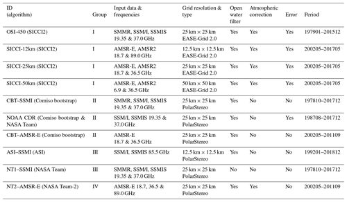
Table 2 Overview of the investigated sea-ice concentration products. The column “ID (algorithm)” holds the identifier we use henceforth to refer to the data record and which algorithm it uses. Group is an identifier for the retrieval concept used. The column “Input data” refers to the input satellite data for the data set. The column “Open water filter” refers to whether weather-related spurious sea-ice concentrations in open water and low-concentration areas are filtered. Weather filters do not remove weather-related noise over areas with near-100 % sea-ice concentrations. The column “Atmospheric correction” refers to correcting the input TBs for a potential inherent weather influence using additional independent weather information. The column “Error” refers to the provision of sea-ice concentration uncertainties, and “Period” is the time period for which we use the data set, given as StartYearStartMonth–EndYearEndMonth.

A considerable number of different algorithms to compute the sea-ice concentration from microwave satellite TB measurements have been developed during the past decades. All exploit the fact that under typical viewing angles (50–55^∘) the difference in microwave brightness temperature, measured at horizontal (h) and vertical (v) polarization, between open water and sea ice is sufficiently large to estimate sea-ice concentration. Whether or not a given algorithm is accepted by the scientific community as a candidate for computing a climate data record (CDR) depends among other things on the length of the available satellite raw data record, spatial and temporal resolution, quantification of uncertainties, and sensitivity to noise, which might introduce artificial trends (e.g. Tonboe et al., 2016; Lavergne et al., 2019).

Several inter-comparison studies were carried out to assess the quality of the sea-ice concentration obtained with different algorithms (e.g. Andersen et al., 2007; Ivanova et al., 2014, 2015; Beitsch et al., 2015; Comiso et al., 2017a). Two different kinds of such inter-comparisons exist. One kind deals with an inter-comparison of sea-ice cover products of a certain number of algorithms without incorporating independent information of the sea-ice cover. Such inter-comparisons provide very valuable information about inter-product consistencies in the overall sea-ice concentration distribution and in sea-ice area and extent time series and trends. They also reveal differences, for instance, with respect to the representation of the seasonal cycle or with respect to regional differences between sea-ice concentration estimates. Inter-comparisons of this kind are Ivanova et al. (2014) and Comiso et al. (2017a). These studies, however, do not provide information about how accurate a sea-ice concentration product is. The other kind of algorithm inter-comparison study deals with the comparison of the satellite sea-ice concentration with independent data. These can be ship-based observations, or sea-ice concentration estimates derived from independent satellite observations, for instance, in the optical frequency range or with active microwave sensors such as synthetic aperture radar (SAR). Inter-comparisons of this second kind seldom involve more than one to two algorithms (e.g. Wiebe et al., 2009; Meier, 2005; Comiso et al., 1997; Comiso and Steffen, 2001; Markus and Dokken, 2002; Kern et al., 2003; Cavalieri et al., 2010; Spreen et al., 2008). Exceptions to this are Andersen et al. (2007), who compared seven different algorithms with ship-based sea-ice cover observations and SAR imagery for the high Arctic, and Beitsch et al. (2015), who compared six different algorithms with ship-based sea-ice cover observations in the Antarctic. Both these studies each focused on one hemisphere only. The work of Andersen et al. (2007) is based on comparably old versions of the algorithms and products. In the present paper, we inter-compare the newest available versions of the sea-ice concentration algorithm and products used in both studies, including three CDRs. We perform our evaluation for both hemispheres. Additionally, we take advantage of a recently published new calibration–validation data package (see Sect. 2.2).

This paper is the first of a series of papers in which we are going to present and discuss results of a systematic evaluation of 10 sea-ice concentration products (see Sect. 2). We want to provide users and algorithm developers with new information about the accuracy and precision of this suite of products, some of which are widely used in the climate research community. In this paper, we present the sea-ice concentration products used. We focus on differences in sea-ice concentration, area, and extent and on inter-comparisons with near-100 % reference sea-ice concentrations and with a large suite of ship-based manual visual observations of the sea-ice conditions. The second paper is going to focus on an inter-comparison with sea-ice parameters derived from Moderate Resolution Imaging Spectroradiometer (MODIS) satellite observations in the Arctic. The third paper is going to focus on presenting and discussing results of an inter-comparison with sea-ice concentrations computed from Landsat satellite visible imagery.

In the following Sect. 2, we introduce the sea-ice concentration data sets and ancillary data used as input. This section further describes the preparation of the ancillary data and inter-comparison steps. Section 3 illustrates how the sea-ice concentration products compare with each other in terms of multi-annual monthly average sea-ice concentration as well as sea-ice area and extent. In Sects. 4 and 5, we show the results of the inter-comparison against a near-100 % reference data set and against ship-based sea-ice observations, respectively. Section 6 covers a discussion, an outlook, and conclusions.

2 Data and methodologies

2.1 Sea-ice concentration data sets

For this study, we consider 10 different sea-ice concentration products (Table 2, with more details in Appendices A–F). There are many more algorithms and products available than we are using here; see e.g. Ivanova et al. (2015). The main criteria for our choice of algorithms and products are (1) length of the product time series, (2) grid resolution, and (3) accessibility and sustained production. We exclude products with less than 10-year coverage and/or with a finer grid resolution than 12.5 km. Following Table 2 we comment on several specific issues that are important for the correct interpretation of sea-ice concentration products, namely the grid resolution, the land spillover correction, the weather/open water filter, and the sea-ice concentration distributions around 0 % and 100 %.

We group the products according to their concept for sea-ice concentration retrieval (Table 2, column “Group”). Group I contains the four European Organisation for the Exploitation of Meteorological Satellites-Ocean and Sea Ice Satellite Application Facility – European Space Agency-Climate Change Initiative (EUMETSAT OSI SAF and ESA CCI) products. Group II contains the Comiso bootstrap (CBT) algorithms, which are CBT–SSMI (Special Sensor Microwave/Imager), CBT–AMSR-E (Advanced Microwave Scanning Radiometer aboard Earth Observation Satellite), and National Oceanic and Atmospheric Administration (NOAA) CDR (the third is a combination of CBT–SSMI and NASA Team (NT1)–SSMI but is clearly dominated by CBT–SSMI). NT1–SSMI and Artist Sea Ice (ASI)–SSMI are assigned to group III. These algorithms follow a different concept to retrieve the sea-ice concentration where the sea-ice concentration is mainly based on a brightness temperature polarization difference. Finally, the enhanced NASA Team (NT2)–AMSR-E is assigned to group IV; its concept to derive sea-ice concentrations via a lookup table and modelled atmospheric profiles is fundamentally different from the other nine algorithms.

2.1.1 Grid resolution

Given grid resolutions apply to every grid cell for group I products since their EASE-Grid has equal area of all grid cells (Appendix A). For all other products which are provided on a polar-stereographic grid (Appendices B–F), the grid resolution is true at 70^∘ latitude (see also Peng et al., 2013). For the computation of sea-ice area and extent (Sect. 3), we take this difference in grid cell area into account and use the respective files of the grid cell areas provided by NSIDC (ftp://sidads.colorado.edu/pub/DATASETS/brightness-temperatures/polar-stereo/tools/geo-coord/grid, last access date: 26 September 2018).

2.1.2 Land spillover correction

The difference in brightness temperatures observed over open water (low) and land (high) combined with the size of the field of view of several kilometres to a few tens of kilometres can cause spurious sea-ice concentrations to appear along coasts (e.g. Lavergne et al., 2019). Various methods to reduce this so-called land spillover effect are applied in all products (Cavalieri et al., 1999; Cho et al., 1996; Maass and Kaleschke, 2010). For ASI–SSMI (Appendix B), reduction of land spillover effects is carried out for both the ASI algorithm and the NASA Team algorithm product used over open water. For NOAA CDR (Appendix F), the reduction of land spillover effects is applied separately to both input data sets before merging (Meier and Windnagel, 2018). In this paper, we do not further correct potential differences between the 10 products caused by this effect.

2.1.3 Weather/open water filter

The two standard weather filters based on brightness temperature gradient ratios at 19, 22, and 37 GHz, which mitigate noise due to atmospheric moisture and wind-induced roughening of the ocean surface (Cavalieri et al., 1995, 1999), are applied in the products NT1–SSMI and NT2–AMSR-E. In the products CBT–SSMI and CBT–AMSR-E, spurious sea-ice concentrations caused by weather effects are filtered using the same frequencies as mentioned above but applying a bootstrap technique (Comiso and Nishio, 2008). For NOAA CDR (Appendix F), the above-mentioned weather filters are applied before the merge (Meier and Windnagel, 2018). In the two National Aeronautics and Space Administration Goddard Space Flight Center (NASA GSFC) (Appendices C, D) sea-ice concentration products, i.e. NT1–SSMI version 1 and CBT–SSMI version 3, weather effects are reduced by screening of input brightness temperatures, application of the above-mentioned weather filters, and some additional manual correction (Meier and Windnagel, 2018; Peng et al., 2013, https://nsidc.org/data/g02202/versions/3, last access: 7 February 2019, https://nsidc.org/data/nsidc-0051, last access: 7 February 2019, and https://nsidc.org/data/nsidc-0079, last access: 7 February 2019). In the ASI–SSMI product no specific weather filter is applied to the ASI algorithm itself. However, ASI algorithm sea-ice concentrations are set to 0 % where NASA Team algorithm sea-ice concentration values are < 30 % (see Appendix B). Because the above-mentioned two weather filters are applied to the NASA Team sea-ice concentration, the ASI–SSMI product implicitly contains a weather filter as well (Ezraty et al., 2007). Note that the 5 d median filter used for the ASI–SSMI product used here (Kern et al., 2010) not only removes remaining spurious sea ice over open ocean but also reduces weather-induced elevated sea-ice concentrations along the ice edge. In the group I products a dynamic open water filter is applied. It is based on the quoted standard weather filters but takes into account changes in filter efficiency due to changes in the frequencies between the different sensors, for instance between SMMR and SSM/I. Also, it does not use the channels close to 22 GHz. All weather filters may in addition to the spurious ice also remove real ice along the ice edge. All 10 products apply a monthly varying climatological sea-ice cover mask to erase spurious sea ice at low latitudes.

We investigate the temporal consistency of the weather filters. For this we focus on the sea-ice concentration interval ]0.0 %, 30.0 %]; i.e. we exclude grid cells set to exactly 0.0 % by the weather filter. Then, for each day of the month, we identify the 5th percentile of all gridded sea-ice concentrations falling into the above-mentioned interval. Subsequently, we average over the month. We look at two aspects. First, it is desirable that these time series are mostly stable across the time period covered by a given data record, indicating that the weather filter cuts the sea-ice edge evenly across inter-annual variability and changes of frequencies. Second, it is also desirable that the weather filter cuts “well below” the 15 % SIC threshold that is commonly used in the computation of the sea-ice extent (SIE) (e.g. Gloersen et al., 1992; Meier et al., 2014; Comiso et al., 2017a). We choose the 5th percentile (and not a minimum value) to obtain less noisy time series. We plot examples of these time series for all 10 products in Figs. 1 and 2 for the Arctic and Antarctic, respectively. For the Arctic we use March (Fig. 1a) and September (Fig. 1g); for the Antarctic we use September (Fig. 2a) and February (Fig. 2g). In addition to the time series, we also plot the cumulative distribution of the daily sea-ice concentrations of the range ]0.0 % to 30.0 %] for the respective month for the year 2004 as an example for CBT–SSMI, OSI-450, NT1–SSMI, ASI–SSMI, and NT2–AMSR-E.

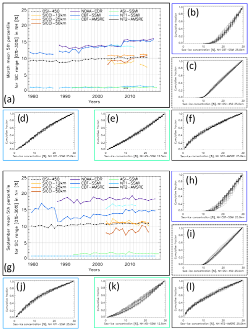
Figure 1 Time series of the monthly mean 5th percentile sea-ice concentration of the range ]0.0 % to 30.0 %] for the Arctic in (a) March and (g) September for all 10 products. Panels (b–f) and (h–l) show daily cumulative sea-ice concentration distributions of five selected products in these two months, respectively, in a sample year: 2004. See Table 2 for the time periods with data from the respective products.

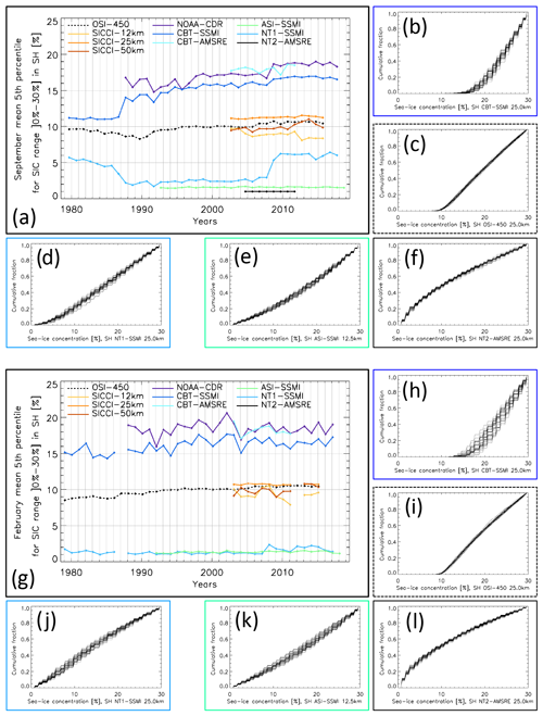
Figure 2 Time series of the monthly mean 5th percentile sea-ice concentration of the range ]0.0 % to 30.0 %] for the Antarctic in (a) September and (g) February for all 10 products. Panels (b–f) and (h–l) show daily cumulative sea-ice concentration distributions of five selected products in these two months, respectively, in a sample year: 2004. See Table 2 for the time periods with data from the respective products.

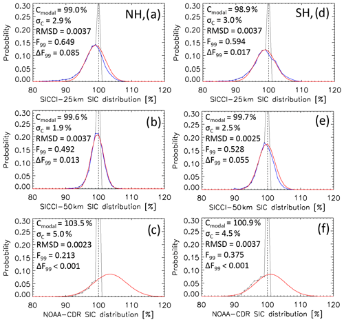
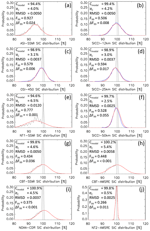
Figure 3 Examples of the sea-ice concentration distribution at near-100 % reference sea-ice concentration locations. Black symbols and lines show values cut off at 100 %; blue lines denote the original distribution (for SICCI-25km and SICCI-50km only); red lines denote the distribution resulting from the Gaussian fit to values of the distribution ≤ 99 %. In each panel, the modal sea-ice concentration (centre of the Gaussian fit: C_modal), the standard deviation of the fit σ_C and fit parameters with respect to the fraction of the distribution ≤ 99 % (F₉₉, ΔF₉₉; see text for more explanation), and the root-mean-squared difference (RMSD) between original and fitted probability are given. (a–c) Arctic; (d–f) Antarctic. See Appendix H for Figs. H1 and H2 containing plots of this kind for all 10 products.

We find little inter-annual variation in the monthly mean percentile sea-ice concentration over time, particularly for OSI-450 and SICCI-25km (see also Lavergne et al., 2019). Changes as caused due to a switch in sensor remain below 1 %. On average, the 5th percentile sea-ice concentration is < 12 %, which ensures that the enhanced open water filter applied in these two products barely influences computation of SIA and SIE. For group II products, these monthly mean 5th percentile sea-ice concentrations are considerably larger and sometimes exceed 15 %. Additionally, the time series for CBT–SSMI and NOAA CDR reveal larger inter-annual variations than OSI-450, inter-sensor transitions (e.g. in 1987–1988 changing from SMMR to SSM/I, Fig. 1g); and in 2007–2008 changing from SSM/I to SSMIS, Fig. 1a) leading to trends in the percentile time series. Compared to OSI-450 and SICCI-25km, for NOAA CDR we find the following. (1) The sea-ice concentration at which the weather filter applies varies seasonally. For instance, in the year 1996, the mean 5th percentile of sea-ice concentrations within the interval ]0 %, 30 %] is 14 % for the Arctic in March but 17 % in September, and for the Antarctic it is 16 % in September but 18 % in February. OSI-450 cuts at 10 % and SICCI-25km cuts at 11 % in these months, and for both hemispheres. (2) The inter-annual variation in the sea-ice concentration at which the filter applies is larger for NOAA CDR than for OSI-450 and SICCI-25km. The time series for NT1–SSMI, ASI–SSMI, and NT2–AMSR-E, in contrast, have very low (∼ 1 %) monthly mean 5th percentile sea-ice concentration values with little or no inter-annual variation.

In the plots showing the daily cumulative fraction for the year 2004, which exemplifies the typical cumulative fraction, we find a cumulative distribution with a first increasing, later merely constant slope with no sea-ice concentrations below ∼ 10 % and ∼ 8 % for CBT–SSMI and OSI-450, respectively (panels b, c, h and i in Figs. 1 and 2). This agrees with the application of the open water filter presented in Lavergne et al. (2019). For NT1–SSMI and NT2–AMSR-E, in contrast, we find a substantial amount of near-0 % sea-ice concentrations (panels d, f, j and l in Figs. 1 and 2). This suggests that while a weather filter is applied (according to the documentations) there are still concentrations near 0 % left. We checked this by looking at the respective daily sea-ice concentration maps. Both products reveal a considerable number of grid cells with < 5 % sea-ice concentration along the ice edge. All but the group I products (see Table 2) only provide integer sea-ice concentration values. At the near-0 % end of the sea-ice concentration distribution these products have sea-ice concentrations of 0 %, 1 %, 2 %, and so forth. The number of NT2–AMSR-E sea-ice concentration values of 1 % exceeds the 5th percentile most of the time, which is the explanation for why most NT2–AMSR-E values are missing in the time series in plots (a) and (g) of Figs. 1 and 2. We take the results shown in these two figures into account when discussing the results presented in Sect. 3.

2.1.4 Distribution around 100 %

A considerable fraction of this paper focuses on the evaluation near 100 % sea-ice concentration. Sea-ice concentrations are retrieved from satellite microwave brightness temperatures using a geophysical algorithm, usually involving tie points. Tie points are typical signatures, e.g. brightness temperatures, or parameters derived from these, of ice (SIC: 100 %) and open water (SIC: 0 %). Because of the natural variability of the surface properties of 100 % sea ice relevant for its microwave remote sensing, one fixed tie point value for 100 % sea ice, even if retrieved daily, can only be an average representation of these properties. In other words, 10 different kinds of 100 % sea ice can cause 10 different brightness temperatures. As a result, a retrieved sea-ice concentration naturally varies around 100 %. This means even though the actual sea-ice concentration is exactly 100 % the retrieved one could be, for example, 97 % or 100 % or 103 %. While the group I products retain the naturally retrieved sea-ice concentration, the others do not; in all group II to group IV products (see Table 2) sea-ice concentrations are truncated at 0 % and 100 %; i.e. values < 0 % are set to 0 % and values > 100 % are set to 100 %. Figure 3 illustrates the sea-ice concentration distribution at the locations of the near-100 % sea-ice concentration reference data set (see Sect. 2.2) for SICCI-25km, SICCI-50km, and NOAA CDR for the Arctic (panels a–c) and the Antarctic (panels d–f).

We use a Gaussian fit to reconstruct the true distribution of the sea-ice concentration retrieval around 100 % for group II and III products. The methodology is tested on the group I products. This is done by finding that Gaussian curve which provides the lowest root-mean-squared difference (RMSD) to the sea-ice concentration distribution for values ≤ 99 %, i.e. basically the left-hand side of the histograms shown in Fig. 3. For the fitting process, we also take into account the fraction of sea-ice concentrations ≤ 99 % relative to the entire count of valid sea-ice concentrations: F₉₉. The difference between original F₉₉ and F₉₉ resulting from the Gaussian fit, ΔF₉₉, has to be < 0.1. We allow a maximum RMSD value of 0.0125. We first binned SICCI-25km and SICCI-50km sea-ice concentration values to integer values to be consistent with the other products. Figure 3a, b and d, e illustrate that the fits (red) agree well with the originally retrieved SICCI-25km and SICCI-50km sea-ice concentrations (blue) with modal values slightly below 100 %. Figure 3c, f illustrate how well the Gaussian fit matches the original sea-ice concentration distribution for sea-ice concentrations ≤ 99 % for NOAA CDR as an example. Here the modal sea-ice concentrations of the Gaussian fit are larger than 100 %: 103.5 % for Northern Hemisphere (NH, Fig. 3c) and 100.9 % for Southern Hemisphere (SH, Fig. 3f). In addition, the Gaussian curve is broader than for SICCI-25km and SICCI-50km, resulting in larger values for the standard deviation. We also note that F₉₉ is ∼ 0.6 and ∼ 0.5 for SICCI-25km and SICCI-50km, respectively, but only ∼ 0.2 and ∼ 0.4 for NOAA CDR. We take the information from Fig. 3 into account when interpreting the results presented in Sects. 4 and 5. We refer to Appendix H for the full set of sea-ice concentrations and Gaussian fits obtained for all 10 products in both hemispheres.

Figure 4 Illustration of the typical distribution of near-100 % SIC reference data by means of the co-located OSI-450 sea-ice concentration for (a, b) the Arctic and (c, d) the Antarctic in a year with good (a, c) and poor (b, d) data coverage.

2.2 The near-100 % sea-ice concentration reference data set

For the evaluation of the 10 products at 100 % sea-ice concentration (see Sect. 4), we use the Round Robin Data Package version 2 (RRDP2) near-100 % reference sea-ice concentration data set developed within the ESA Sea_Ice_cci and European Union “Spaceborne observations for detecting and forecasting sea ice cover extremes” (EU-SPICES) projects (Pedersen et al., 2019). In short, for this reference data set, areas of ∼ 100 % sea-ice concentration are found by identifying areas of interest (AOIs) of approximately 100 km × 100 km with net convergence in the ice drift pattern on two consecutive 1 d periods. Information about convergence is derived from the PolarView/MyOcean/CMEMS ice drift data set derived from Envisat ASAR, RADARSAT-2 SAR, and Sentinel-1 SAR imagery. By choosing AOIs for regions with high concentrations, near-100 % sea-ice concentration can be assured (e.g. Kwok, 2002; Andersen et al., 2007) in winter. Each AOI contains up to a hundred 10 km × 10 km cells for which the SAR ice drift is computed. The number of cells depends on SAR image coverage. Convergence in the ice drift pattern results in a decrease in the total area of these cells. A cell is included in the data set of ∼ 100 % sea-ice concentration if the area reduction between day 1 and day 2 is between 0.4 % and 1.5 % and if more than 40 % of the AOI contains cells with such an area reduction. The RRDP2 near-100 % sea-ice concentration reference data set contains the AOI centre geographic latitude and longitude, time, total sea-ice concentration (100 %), and AOI average area reduction due to net ice convergence. It is available for the years 2007 through 2015 for both hemispheres.

We cannot provide a definite uncertainty for this reference data set but for its production. We combine a suite of measures to ensure high precision and close-to-zero bias (high accuracy). The drift–convergence selection is based on convergence on two consecutive days of 1 d drift. During winter, i.e. November through March (Arctic) and May through September (Antarctic), this is assumed to ensure that all openings existing on day 0 (prior to the two convergence days) are closed by convergence or refrozen. The refreezing assumption is the reason for the product quality to be higher during winter when openings rapidly refreeze than during summer when openings may not freeze up. There is no prior assumption of the initial ice concentration (on day 0), but the ice drift product requires quite high concentrations for the 2-D cross correlation to work. Andersen et al. (2007) reported a sea-ice concentration standard deviation of ∼ 1 % for cold-season high-resolution high-quality SAR image classification and an accuracy of 2 % for ice-water SAR image classification from ice analysts without additional drift–convergence information. Based on our above-mentioned measures and the results of Andersen et al. (2007), we can state estimated values for precision (∼ 1 %) and accuracy (< 0.5 %) for our reference data set.

We co-locate the sea-ice concentrations of the 10 products with the selected AOI grid cells by computing the minimum distance between AOI grid cell centre and grid cell centre of the respective sea-ice concentration product. For this step, we convert the geographic coordinates of all data sets into Cartesian coordinates taking into account the different projections. Figure 4 illustrates the spatial distribution of selected AOIs for both hemispheres for two different years by showing the co-located OSI-450 sea-ice concentration. We give an example of a typical “good distribution” (Fig. 4a, c) and of a typical “poor distribution” (Fig. 4b, d). The RRDP2 near-100 % sea-ice concentration reference data set contains basically no AOIs in the eastern Antarctic because of the lack of SAR image coverage required for the ice drift product used to generate this RRDP2 data set.

We evaluate the products at their native grid resolution without applying any spatial averaging. For each product, we compute the mean difference “product minus 100 %” and its standard deviation as well as the cumulative distribution function of the differences.

2.3 Ship-based visual sea-ice cover observations

According to the Antarctic Sea Ice Processes & Climate (ASPeCt) protocol (http://www.aspect.aq, last access: 18 February 2019; Worby and Allison, 1999; Worby and Dirita, 1999; see also Worby et al., 2008) and the Ice Watch/ASSIST (Arctic Ship-based Sea-Ice Standardization) protocol (http://icewatch.gina.alaska.edu, last access: 5 March 2019), ship-based observations of the sea-ice conditions shall be carried out every hour, at least every second hour, during daylight conditions while the ship is traversing the sea ice. Observations shall be carried out from the ship's bridge for an area of about 1 km around the ship and shall report ice conditions as follows: total ice concentration, type of openings, concentration, thickness, ridge fraction and height, and snow depth and type for up to three ice types. All ship-based visual observations used here result from manual, non-automated observations.

For our evaluation of the 10 products with respect to ship-based visual observations of the sea-ice conditions (see Sect. 5), we use about 15 000 individual observations. About ∼ 7000 of these were carried out in the Antarctic (ASPeCt) and ∼ 8000 in the Arctic (Ice Watch/ASSIST). A substantial fraction of the Antarctic observations (until 2005) is available via http://www.aspect.aq (last access: 18 February 2019, Worby et al., 2008). The more recent observations were collected from various sources (e.g. PANGAEA, ACE-CRC, AWI; see also Beitsch et al., 2015) and merged with the existing ASPeCt data. The majority of the ASSIST data are taken from the data portal http://icewatch.gina.alaska.edu (last access: 5 March 2019). Additional sources for ASSIST data are PANGAEA (for Polarstern cruises before Ice Watch/ASSIST), the Arctic Data Center of the NSF (https://arcticdata.io/catalog/#data, last access: 5 March 2019), and the data archive of the Bering Sea Ecosystem Study (BEST): https://www.eol.ucar.edu/projects/best/ice.shtml (last access: 5 March 2019). All data are standardized; i.e. the ASCII format data files containing the observations use similar formats for all variables and missing data. The data are also manually quality checked for outliers. For the comparison presented in this paper, we use all ASPeCt and Ice Watch/ASSIST observations from the period June 2002 through December 2015 (Kern, 2019).

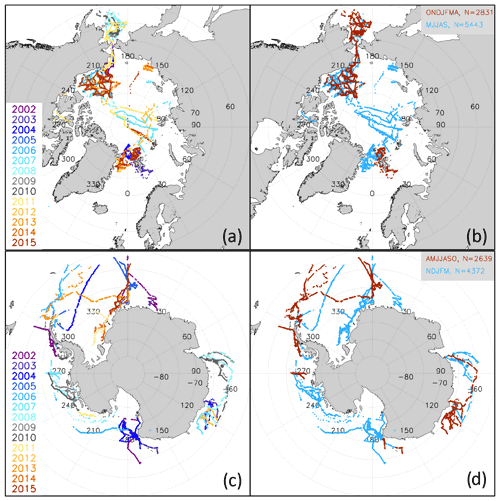
Figure 5 Spatio-temporal distribution of the ship tracks for (a, b) the Arctic and (c, d) the Antarctic from which ship-based visual observations of the sea-ice cover were used. Panels (a, c) illustrate the years, and panels (b, d) distinguish between winter (red) and summer (cyan) months.

Figure 5 summarizes the locations of the ship-based observations used in this paper, separately for the Arctic (Fig. 5a, b) and the Antarctic (Fig. 5c, d). For both hemispheres, just comparably small regions contain such observations. Figure 5a, c illustrate that some regions were visited during several years, while others were visited just once or twice during the 13-year period considered. The seasonal distribution (Fig. 5b, d) illustrates that the more central (Arctic) or southern (Antarctic) regions were only visited during summer months due to harsh winter conditions and missing daylight for these regions.

We co-locate the sea-ice concentrations of the 10 products with the selected ship-based observations by computing the minimum distance between geographic location of the ship-based observation and the grid cell centre of the respective sea-ice concentration product. For this step, we convert the geographic coordinates of all data sets into Cartesian coordinates taking into account the different projections of the sea-ice concentration products. Following the co-location, we average over all ship-based and all satellite-based sea-ice concentration values, including reports of open water, i.e. 0 % concentration, of 1 d following the approach of Beitsch et al. (2015). This results in a comparison of along-ship-track daily average sea-ice conditions. Data pairs with fewer than three ship-based observations per day are discarded. The results of the comparison between ship-based and satellite-based sea-ice concentration are solely based on these daily average sea-ice concentrations. Note that all satellite-based data are used at their native grid resolution.

The ship-based and satellite-based sea-ice concentration data sets are inter-compared (Sect. 5) by means of scatterplots and linear regression analysis and statistics separately for summer data, winter data, and data of the entire year. Summer comprises the months May through September for the Arctic and the months November through March for the Antarctic; winter comprises the remaining months. In the scatterplots, we compare the daily average sea-ice concentrations and additionally compute averages of the satellite-based sea-ice concentration after binning the ship-based data into 5 % wide bins (0 % to 5 % and 95 % to 100 %) and 10 % wide bins (sea-ice concentrations between 5 % and 95 %) and vice versa. We compute the overall average sea-ice concentration difference and its standard deviation and perform a linear regression analysis based on the daily average and the binned data.

Figure 6 Arctic sea-ice area (a, b) and extent (c, d) computed in (a, c) winter (March) and (b, d) summer (September) from the sea-ice concentration data sets used. See Table 2 for start and end months of the respective time series.

3 Inter-comparison of sea-ice area, extent, and distribution

We follow Ivanova et al. (2014) and begin our inter-comparison with time series of the sea-ice area (SIA) and sea-ice extent (SIE) (Sect. 3.1 and 3.2) derived from monthly mean sea-ice concentration. The monthly mean sea-ice concentration is derived for every product at the native grid and grid resolution using data of all days of a month of the entire sea-ice concentration range including 0 %. SIE is computed by summing over the grid cell area with > 15 % sea-ice concentration. SIA is computed by summing over the ice-covered portion of the grid cell area with > 15 % sea-ice concentration. By using this threshold, we follow Gloersen et al. (1992) and numerous SIA and SIE inter-comparison studies. We compare SIA and SIE time series for the entire period for which we have data from the respective products at the time of the analysis. We exclude sea-ice concentrations estimated for lakes and other inland waters. We fill the circular area with missing data around the pole caused by the satellite orbit inclination and swath width with a constant sea-ice concentration value of 98 %. Andersen et al. (2007) found a mean sea-ice concentration of ∼ 98 % from a comparison of cold-season passive microwave and synthetic aperture radar observations in the high Arctic. They noted a smaller value of ∼ 95 % in summer. Both values are confirmed by Kern (2018, http://icdc.cen.uni-hamburg.de/fileadmin/user_upload/ESA_Sea-Ice-ECV_Phase2/SICCI_Phase2_SIV-Retrieval_Report_v02.pdf, last access: 6 September 2019). Using 98 % instead of 95 % during summer results in an overestimation of the SIA of about 10 000 km², a small value compared to other sources of biases for the SIA during summer. This filling is applied to the Arctic and only to the products at polar-stereographic projection. This area is already interpolated spatially in the four group I products. As described in Lavergne et al. (2019), these products contain a fully filtered and truncated (to the range [0.0 % … 100.0 %]) version and a non-filtered, non-truncated version of the sea-ice concentration. The latter contains the naturally retrieved sea-ice concentrations, i.e. also values < 0 % and > 100 % (see Sect. 2.1.3), and no weather filters are applied (see Sect. 2.1.3). We use the fully filtered and truncated version. Without the truncation the SIA of the group I products increases slightly, while the SIE does not change because the number of grid cells covered with > 15 % sea ice is not influenced by the truncation (not shown).

Figure 7 As Fig. 6 but for the Antarctic.

We complement these SIA and SIE time series with maps of the multi-annual average sea-ice concentration difference for selected months for the AMSR-E measurement period: June 2002 to September 2011 (Sect. 3.3 and 3.4). We choose this period to be able to compare all 10 products for a similarly long time period. For these maps, we first re-grid the monthly mean sea-ice concentrations of all products, except SICCI-50km, onto the EASE-Grid version 2.0 with 50 km grid resolution using bilinear interpolation. Then we compute the multi-annual average sea-ice concentration for each month from which we subsequently calculate an ensemble median and the difference product minus ensemble median.

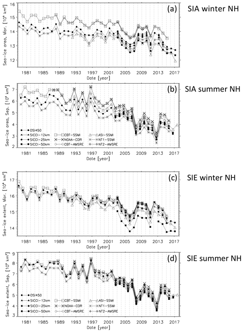
3.1 Arctic sea-ice area and extent time series

The SIA and SIE time series for the Arctic reveal a very similar overall development for the products extending back into the 1980s and 1990s (Fig. 6). This applies to (i) the overall negative trend in both quantities; (ii) the inter-annual variability as, for instance, during 1991–1997 and around 2007 and 2012 for SIA and SIE in September (Fig. 6b, d), or in 2011 for the relative minimum in March SIA and SIE (Fig. 6a, c); and (iii) the ranking between the products. NOAA CDR and CBT–SSMI provide the largest SIA and SIE in both March and September. NT1–SSMI provides the lowest SIA and SIE in September, while in March we find SIA and SIE from ASI–SSMI to be even lower. It is obvious that differences between products are smaller for SIE than for SIA as was also shown by Ivanova et al. (2014). For the AMSR-E period, when SIA and SIE of all 10 products are available, the inter-annual variation is similar for all 10 products. We find ESA CCI products, CBT–AMSR-E, and NT2–AMSR-E fall into the ranges of SIA and SIE given by the other products. An exception to this is SICCI-50km, which clearly provides the lowest SIE of all products in March (Fig. 6c). We will discuss this finding in Sect. 3.3.

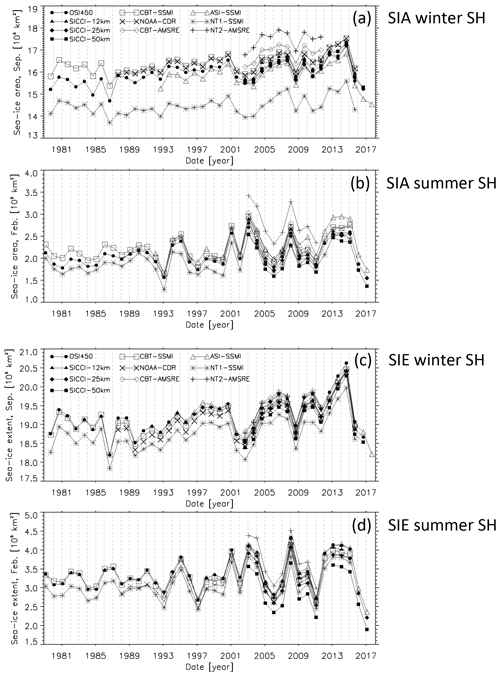
3.2 Antarctic sea-ice area and extent time series

The SIA and SIE time series for the Antarctic reveal a similar overall development for products extending back into the 1980s and 1990s (Fig. 7). This applies to (i) the overall positive trend until 2015 in both quantities; (ii) the inter-annual variability, for instance, during 2000–2003 for SIA and SIE in February (Fig. 7b, d), or in 2008 for the relative minimum in SIA and SIE in September (Fig. 7a, c); and (iii) the ranking between products. NOAA CDR and CBT–SSMI provide the largest SIA while NT1–SSMI provides the smallest SIA, being ∼ 1.8 million km² and 300 000 km² below the SIA of NOAA CDR and CBT–SSMI in September and February, respectively. OSI-450 and CBT–SSMI provide the largest SIE, exceeding the smallest SIE of NT1–SSMI by ∼ 500 000 km² and ∼ 300 000 km² in September and February, respectively (Fig. 7c, d). Inter-product differences are larger for SIA than SIE in September but not in February. For the AMSR-E period, the inter-annual variation is similar for all 10 products. In September, SIA and SIE of the ESA CCI products mostly fall between ASI–SSMI and OSI-450 (Fig. 7a, c). In February (Fig. 7b, d), SICCI-50km provides the smallest overall SIA and SIE while the SICCI-12km and SICCI-25km products agree closely with OSI-450. In contrast to the Arctic (compare Fig. 6), NT2–AMSR-E clearly provides the largest SIA in September and February (Fig. 7a, b). NT2–AMSR-E provides the largest SIE in February as well (Fig. 7d).

Figure 7c contains an example of discontinuities caused by the application of weather filters not adapted to sensor changes. Wintertime Antarctic OSI-450 and CBT–SSMI SIE agree with each other for the SMMR period. After 1987 the CBT–SSMI SIE is lower than the OSI-450 SIE by ∼ 150 000 km². This corresponds to the area of one-quarter of all 25 km grid cells at a latitude of 60^∘ S, the approximate average location of the Antarctic sea-ice edge in September. This change in SIE is concomitant with a jump in the weather filter sea-ice concentration from 11 % to 14 % (Fig. 2a). It is noteworthy that the 23.0 GHz channels of the SMMR instrument were highly unstable from launch and eventually ceased to function on 11 March 1985 (Njoku et al., 1998). Thus, the water vapour part of the “classic” weather filter is unreliable in the early decade of the satellite data record. This is solved in the OSI-450 product by relying on explicit atmospheric correction of the brightness temperatures using – among others – water vapour fields from atmosphere reanalysis (see Lavergne et al., 2019). Another example of this kind (not shown) is a shift between OSI-450 SIE and NOAA CDR SIE by 50 000 to 100 000 km² between 2007 and 2008. This shift is concomitant with a discontinuity in the weather filter sea-ice concentration for NOAA CDR in March (Arctic, Fig. 1a) and September (Antarctic, Fig. 2a) during the transition from 2007 to 2008. This corresponds to when SSMIS (F17) is processed instead of SSM/I (F15). OSI-450 exhibits no discontinuity here.

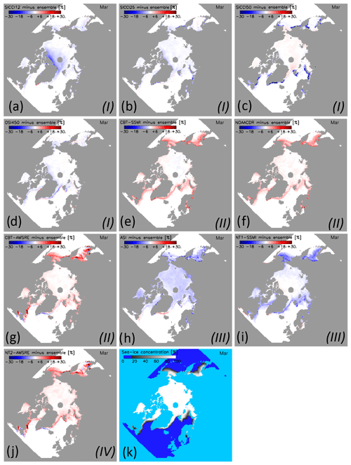
Figure 8 (a–j) Maps of the difference between the multi-annual average monthly SIC of the individual algorithms and the 10-algorithm ensemble median multi-annual average monthly SIC (k) for the Arctic in winter (March) 2003–2011. Differences are only computed for sea-ice concentration of both data sets > 15 %. Roman numbers I to IV denote the group assigned to the respective algorithm (see text for details).

3.3 Arctic sea-ice concentration distribution differences

In March, the difference between the sea-ice concentration of an individual product and the ensemble median of all 10 products (Fig. 8) remains within ±5 % over most of the Arctic Ocean, except for ASI–SSMI (Fig. 8h) and SICCI-12km (Fig. 8a). The largest differences between individual products and the ensemble median are located in the peripheral seas. Group II and IV (see Table 2) products have more sea ice than the ensemble median (Fig. 8e–g, j); differences can exceed 20 %. NT1–SSMI (Fig. 8i) has less sea ice than the ensemble median with negative differences greater than 10 % or even 15 % in magnitude in all peripheral seas. Differences of OSI-450 or SICCI-25km and the ensemble median are within ±5 % almost everywhere (Fig. 8b, d). SICCI-50km exhibits negative differences greater than 20 % in magnitude along some of the coastlines, e.g. the Labrador Sea, the Irminger Sea, or the coastlines of the Pechora Sea and Barents Sea (Fig. 8c). A careful check of these areas in daily and monthly mean maps of the SICCI-50km sea-ice concentration reveals that for regions with a relatively narrow sea-ice cover stretching along coastlines, the coarse resolution of the 6.9 GHz frequency channel entering the algorithm (see Table 2), in combination with land spillover filter and open water filter, can result in an unwanted complete removal of sea ice from the grid cells of the product. We are confident that this explains the particularly low SICCI-50km SIA and SIE shown in Fig. 6a and c for Arctic SIE in March.

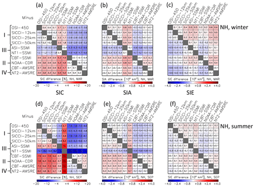
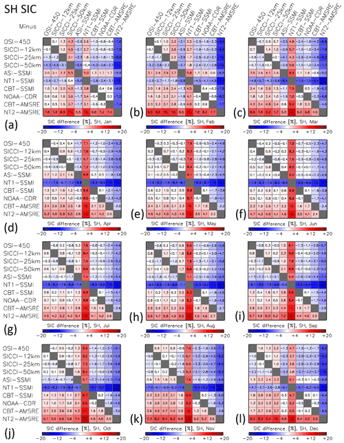
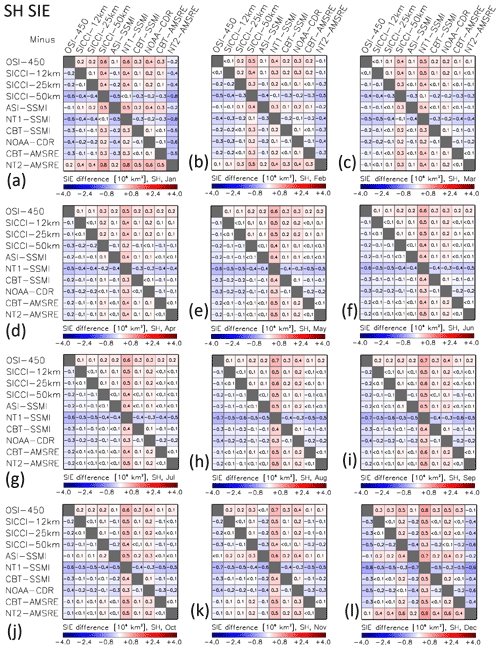
Figure 9 Differences (row minus column) between all 10 products of, from left to right, the average sea-ice concentration SIC, average SIA, and average SIE for the Arctic (NH) in winter (a–c) and summer (d–f). The averages are computed from monthly mean values of the respective months (March, September) of the AMSR-E period June 2002 to September 2011. All data are on the EASE-Grid 2.0 with 50 km grid resolution. The land mask of the SICCI-50km product is applied to all products. Roman numbers I to IV denote groups according to Table 2. For matrices of all remaining months, we refer to Figs. G1–G3 in Appendix G.

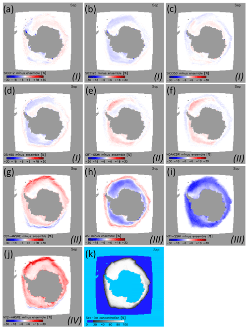
Figure 10 (a–j) Maps of the difference between the multi-annual average monthly SIC of the individual algorithms and the 10-algorithm ensemble median multi-annual average monthly SIC (k) for the Antarctic in winter (September) 2002–2011. Differences are only computed for sea-ice concentration of both data sets > 15 %. Roman numbers I to IV denote the group assigned to the respective algorithm (see text for details).

For the matrices shown in Fig. 9 (and Fig. 12, Appendix G1–G6), we re-grid the monthly mean sea-ice concentration onto the EASE-Grid version 2.0 with 50 km grid resolution using bilinear interpolation, and we apply a common land mask (that of SICCI-50km) to all products. The differences between SIA and SIE values are computed from these gridded 50 km resolution, common land mask products. Figure 9a agrees with the results shown in Fig. 8. In winter (March), sea-ice concentration differences between members of groups I to III are < 1 %. Group III members NT1–SSMI and ASI–SSMI (see Table 2) exhibit less sea ice than the other groups. Group II and IV members exhibit higher sea-ice concentrations than the other two groups in winter and summer (September). In summer (Fig. 9d), sea-ice concentration differences remain < 2 % between members of groups I and II but not within group III, where differences exceed 10 %. We refer to Appendix G for the respective results of the other months.

3.4 Antarctic sea-ice concentration distribution differences

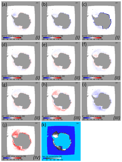
In September (Fig. 10), most products show more sea ice than the ensemble median over high-concentration ice and less sea ice along the marginal ice zone. NT1–SSMI (Fig. 10i) exhibits considerably less sea ice than the ensemble median almost everywhere (see also Fig. 12a). ASI–SSMI (Fig. 10h) exhibits a distribution of sea-ice concentration differences that is reversed compared to most other products. CBT–AMSR-E and especially NT2–AMSR-E (Fig. 10g, j) show more sea ice than the ensemble median for most regions. This is evident in Fig. 12a as well.

Figure 11 As Fig. 10 but in summer (January) 2003–2011.

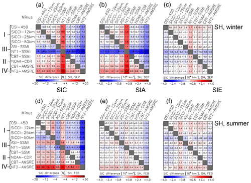
Figure 12 Differences (row minus column) between all 10 products of, from left to right, the average sea-ice concentration SIC, average SIA, and average SIE for the Antarctic (SH) in winter (a–c) and summer (d–f). The averages are computed from monthly mean values of the respective months (September, February) of the AMSR-E period June 2002 to September 2011. All data are on the EASE-Grid 2.0 with 50 km grid resolution. The land mask of the SICCI-50km product is applied to all products. Roman numbers I to IV denote groups according to Table 2. For matrices of all remaining months we refer to Figs. G4–G6 in Appendix G.

In January (Fig. 11), the few, comparably small, high-concentration areas exhibit sea-ice concentration differences mostly below ±5 %. Over the lower-concentration areas, i.e. mainly in the Weddell Sea and the Ross Sea, most products show less sea ice than the ensemble median with differences between 0 % and −6 %. NT1–SSMI has less sea ice while ASI–SSMI and particularly NT2–AMSR-E have more sea ice (see also Fig. 12d). Important to note are the negative differences of ∼ −10 % along most of the Antarctic coast for SICCI-50km (Fig. 11c). Like for the Arctic, the coarse resolution of the 6.9 GHz frequency channels combined with land spillover and open water filters can result in the unwanted removal of sea ice from grid cells (compare Fig. 8c and discussion of it) with the same influence on SICCI-50km SIA and SIE values (Fig. 7b, d). This is also evident in Fig. 12d where SICCI-50km exhibits the largest inter-product differences within group I.

For the results shown in Figs. 6–12 we used the truncated sea-ice concentration values as far as it concerns group I products. Repeating these computations with the non-truncated values, e.g. in September and March, does not change the results with respect to SIE. SIA increases by ∼ 50 000 km² in winter months and there is almost no impact in summer.

3.5 Summary and discussion of sea-ice area and extent findings

The inter-product mean sea-ice concentration differences (Figs. 8–12) are associated with a notable impact on SIA and SIE (Figs. 9 and 12). For summer SIE, inter-product differences are below ∼ 200 000 km² (Arctic, Fig. 9f) and below ∼ 300 000 km² (Antarctic, Fig. 12f) for most products. NT1–SSMI (Arctic) and SICCI-50km, NT1–SSMI, and NT2–AMSR-E (Antarctic) show the largest differences here. For winter SIE, most inter-product differences are below ∼ 200 000 km² for the Antarctic (Fig. 12c); larger differences are mostly found for NT1–SSMI (see also Fig. 7c). For the Arctic (Fig. 9c), inter-product differences range between 100 000 and 600 000 km² and seem to be associated with the type of algorithm and partly also the sensor.

For Arctic winter SIA (Fig. 9b), group III products provide systematically smaller values (by ∼ 400 000 km²) than the other three groups while group II SSMI products provide systematically larger values (by ∼ 300 000 km²). Group I and CBT–AMSR-E and NT2–AMSR-E exhibit the lowest inter-product SIA differences. For Arctic summer SIA (Fig. 9e), group II and IV products agree with each other within 100 000 km² but exceed group I SIA by ∼ 400 000 km². This is equal to 10 % of the summer minimum Arctic SIA. For Antarctic summer SIA (Fig. 12e), NT2–AMSR-E exceeds SIA of all other products by ∼ 400 000 km². This equals 20 % of the summer minimum Antarctic SIA. SIA differences between the other products are almost all < 200 000 km². For Antarctic winter SIA (Fig. 12b), NT2–AMSR-E and NT1–SSMI stand out with very large systematic differences from all other products.

We summarize our findings from the matrices in Figs. 9 and 12 (see also Appendix G1–G6) as follows: (i) absolute and relative (to the respective minimum or maximum value) inter-product differences are smaller for SIE than for SIA. (ii) SIA and SIE derived from products of different algorithms of the same group (see Table 2) may differ considerably. (iii) Inter-product differences for SIA and SIE for the investigated CDRs are, on average, larger for the Arctic than the Antarctic.

We note that the grid resolution of the products is not necessarily compatible with the true spatial resolution because the footprints of the satellite sensor channels used in some of the algorithms are coarser (Table 2). This applies to NT1–SSMI, CBT–SSMI, NOAA CDR, and OSI-450, i.e. the products at 25 km grid resolution based on SMMR, SSM/I, and SSMIS data. For these products, we expect that gradients in the sea-ice concentration are more smeared than for products with a better match between footprint size and grid resolution such as, for instance, CBT–AMSR-E or SICCI-25km. This is illustrated for OSI-450 and SICCI-25km in Lavergne et al. (2019, Fig. 6). For a typical wintertime Antarctic ice edge at 65^∘ S comprising half a compact and half an open sea-ice cover, this difference in the match of true resolution and grid resolution between SSM/I and AMSR-E products would result in a slightly larger SIE (by ∼ 200 000 km²) derived from the SSM/I product. This is because a compact ice edge is smeared more in the SSM/I product, resulting in more grid cells with a sea-ice concentration > 15 %, the threshold used currently to compute SIE. In fact we find that during winter OSI-450 SIE exceeds SICCI-25km SIE by ∼ 100 000 km² in the Arctic (Fig. 9c) and by ∼ 200 000 km² in the Antarctic (Fig. 12c). Since the algorithms used for the sea-ice concentration retrieval for these two products are almost identical, the difference in SIE can well be attributed to the above-mentioned impact of differences between true and grid resolution. The second pair of almost identical algorithms is CBT–SSMI and CBT–AMSR-E. In the Arctic, in winter, CBT–SSMI SIE exceeds CBT–AMSR-E SIE by ∼ 400 000 km² (Fig. 9c) but in the Antarctic CBT–SSMI SIE is smaller than CBT–AMSR-E SIE by ∼ 100 000 km² (Fig. 12c). Differences in the algorithm itself and/or in the weather filter might be the cause. We refer to the discussion at the end of Sect. 3.2 in this context.

4 Comparison with near-100 % SIC reference data set

In this section, we present results of the evaluation of the 10 products at 100 % sea-ice concentration using the data described in Sect. 2.2. We note upfront that caution should be exercised when reporting and interpreting evaluation statistics like bias (mean value minus 100 %) or root-mean-square error near the 100 % end of truncated sea-ice concentration products. This applies to the results presented in this section but also to Sect. 5. First, the bias of truncated products will necessarily be negative or zero (mean value lower than or equal to 100 %), even if the bias of the product was exactly 0 % before truncation. Second, products whose non-truncated distribution is biased high (modal value larger than 100 %) will seemingly achieve better evaluation statistics after truncation because of the accumulation of values > 100 % being folded to exactly 100 %. Both bias and RMSE of these products are smaller than those of products that do not overestimate at 100 % sea-ice concentration. The larger the fraction of truncated values, the better the statistics. The values that accumulate at the 100 % bin in the truncated product are in majority from the above-100 % range of the non-truncated distribution (note the value of F₉₉ in Fig. 3) and improve the evaluation statistics (bias and RMSE). In fact, under the hypothesis that the distribution of the retrieved sea-ice concentration is mostly Gaussian around the modal value before truncation, products with overestimation of the non-truncated distribution can be recognized by their abnormal (with respect to a Gaussian model) accumulation of values exactly at 100 %.

For more discussion and quantification of the error distribution of sea-ice concentration products and algorithms before truncation around 100 % (and around 0 %), see Ivanova et al. (2015).

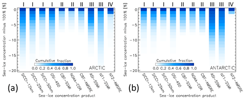
Figure 13 Cumulative distribution of the SIC difference to 100 % at the near-100 % reference SIC locations for all 10 algorithms based on data of the years 2007 through 2011 for (a) the Arctic and (b) the Antarctic. Roman numbers at the top denote product groups (see Table 2).

4.1 Arctic

The distribution of the sea-ice concentration near 100 % is shown for the Arctic for each product in Fig. 13a in the form of the cumulative fraction of the deviation (bias) from 100 %. As expected, the cumulative fraction increases towards 1.0 for all products. Considerable differences between the products are evident. Group I products (see Table 2) exhibit a cumulative fraction between ∼ 0.5 and ∼ 0.7 in bin −1.5 % … −0.5 %. Group II products and NT1–SSMI exhibit substantially lower fractions for this bin: between ∼ 0.2 (NOAA CDR; see also F₉₉ in Fig. 3c) and ∼ 0.4 (NT1–SSMI). Consequently, the change in cumulative fraction to the last bin is between 0.6 and 0.8 for group II and NT1–SSMI but only between 0.3 and 0.5 for group I. The respective F₉₉ values in Fig. 3 and Appendix H suggest that a large portion of the cumulative fraction in the last bin is in fact due to sea-ice concentrations > 100 % being set to 100 % (i.e. truncated). For NT2–AMSR-E, the cumulative fraction increases abruptly from < 0.1 in bin −2.5 % … −1.5 % to ∼ 0.8 in bin −1.5 % … −0.5 %. This behaviour is completely different from all other products and confirms the results of Andersen et al. (2007) and Ivanova et al. (2015). For their inter-comparison of sea-ice concentration algorithms in the high Arctic, Andersen et al. (2007) extended the range within which the NT2 algorithm permits the retrieval of the sea-ice concentration to 120 % in order to be able to properly compare all algorithms with respect to their precision close to 100 %. The original implementation of the NT2 algorithm is constrained to sea-ice concentrations up to 100 %. Ivanova et al. (2015) also aimed to compare the precision of several sea-ice concentration algorithms at 100 % by means of computing the standard deviation of the sea-ice concentration at 100 %. They were, however, unable to obtain standard deviations with comparable statistics because of large positive biases for the NT2 and ASI algorithms and because of the truncation of sea-ice concentrations at 100 %. Only by constructing a reference sea-ice concentration of 75 %, were Ivanova et al. (2015) able to carry out a comparison of the sea-ice concentration standard deviation based on non-truncated sea-ice concentrations.

These cumulative distributions suggest that an inter-comparison of the mean difference to 100 %, i.e. the bias, and its standard deviation, i.e. the precision, should be carried out by means of the Gaussian fit proposed in Sect. 2.1.4. Consequently, the mean sea-ice concentrations of the 10 products shown by the black symbols in Fig. 14a for the Arctic near-100 % reference sea-ice concentration locations are the modal values of the Gaussian fits. The error bars denote 1 standard deviation of this fit around the modal value. The blue symbols and error bars denote the respective mean and 1 standard deviation computed from the non-truncated group I sea-ice concentration products. All values shown here are summarized together with the results obtained from the truncated sea-ice concentration products in Table 3.

Table 3 Inter-comparison results to near-100 % SIC (RRDP2) for the Arctic (see Fig. 14a). The rows “Gaussian” show the mean difference of the modal value of Gaussian fit to satellite SIC ≤ 99 % (compare Fig. 3) minus near-100 % reference SIC (RRDP2 SIC) ± 1 sigma of the Gaussian fit (see Fig. 14a). The rows “Non-truncated” show the mean difference satellite SIC minus RRDP2 SIC ± 1 standard deviation of the difference for SICCI and OSI-450 products. The rows “Truncated” show the mean difference of satellite SIC constrained to a maximum value of 100 % minus RRDP2 SIC ± 1 standard deviation of the difference. All values in these rows are given in percent sea-ice concentration. Values in rows denoting the periods 2007–2015 and 2007–2011 contain the number of valid data pairs. See text for meaning of ^* in the column “NT2–AMSR-E”.

Figure 14a confirms our hypothesis that those products where the cumulative distributions seem to contain a large fraction of sea-ice concentrations larger than 100 % set to 100 % (Fig. 13a), i.e. the group II products, and NT1–SSMI are likely to overestimate the actual sea-ice concentration. The overestimation is particularly high for NOAA CDR with a modal sea-ice concentration of ∼ 103 % (see also Table 3). The group I products exhibit modal sea-ice concentrations that are slightly below and closest to the near-100 % reference. The Gaussian fit also almost perfectly matches the actually observed non-truncated sea-ice concentration for SICCI-50km in terms of the standard deviation (compare blue and black symbols in Fig. 14a and Table 3). The match is less accurate for OSI-450 and SICCI-25km.

In addition, Fig. 14a and Table 3 confirm our hypothesis that the group II products and NT1–SSMI are likely to have a standard deviation that is lowered by truncating sea-ice concentrations to a maximum of 100 %. This is illustrated by the standard deviations of the non-truncated and the truncated sea-ice concentration for group I products (Table 3). Under the assumption that the standard deviation of the Gaussian fit is a better measure of the spread in sea-ice concentrations near (but below) 100 %, we state that the CDRs of group I (SICCI-50km, OSI-450, and SICCI-25km) allow a better precision than group II products. We also confirm the findings of Lavergne et al. (2019) that the group I products are slightly – but significantly – biased low.

For ASI–SSMI and NT2–AMSR-E, the application of a Gaussian fit is potentially not justified given the way sea-ice concentrations are retrieved. ASI–SSMI is non-linear near 100 % (Kaleschke et al., 2001) while no statement about the functional relationship of the input satellite data and the retrieved sea-ice concentrations can be made for NT2–AMSR-E (Markus and Cavalieri, 2000; Brucker et al., 2014). Our analysis, however, results in a reasonable Gaussian fit for ASI–SSMI (see Appendix H, Fig. H1a). We are confident therefore that the values taken from the fit and shown in Fig. 14a and Table 3 can be used. In contrast, the NT2–AMSR-E sea-ice concentration distribution does not allow reasonable application of a Gaussian fit (see Appendix H, Fig. H1j) and we do not report it along with the others in Fig. 14a. We note that Andersen et al. (2007) reported a mean NT2 sea-ice concentration of ∼ 105 % with a standard deviation of ∼ 5 % at near-100 % sea-ice concentrations for their unconstrained version of this algorithm.

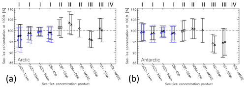
Figure 14 Summary of the results of the inter-comparison to the near-100 % reference SIC (RRDP2) for (a) the Arctic and (b) the Antarctic. Shown for each sea-ice concentration product in black is the centre of the Gaussian fit of the sea-ice concentration ≤ 99 % at the respective RRDP2 locations (see Fig. 4). Bars denote ± 1 standard deviation of the Gaussian fit. For symbol pairs (all products but CBT–AMSR-E and NT2–AMSR-E) the left symbol is based on data of the years 2007–2011 and the right one on data of the years 2007–2015. Blue symbols denote the mean non-truncated sea-ice concentration at the near-100 % reference SIC for OSI-450 and SICCI products; blue bars denote the respective sea-ice concentration standard deviation. Roman numbers at the top denote product groups (see Table 2). No values are shown for NT2–AMSR-E because a Gaussian fit could not be adequately applied.

4.2 Antarctic

For the Antarctic (Fig. 13b), we find more similarities in the cumulative fractions of the deviation (bias) from 100 % than for the Arctic. Common to all products, except NT2–AMSR-E and ASI–SSMI, is a notable step change in the cumulative fraction between bin −1.5 % … −0.5 % and the last bin. This step change is least pronounced for NT1–SSMI and most pronounced for NOAA CDR, exhibiting cumulative fractions of ∼ 0.8 and ∼ 0.4, respectively, in the last bin. Step changes are slightly larger for the two CBT products than for group I products (see also F₉₉ values in Fig. 3d, e). For ASI–SSMI the cumulative fraction levels off before the last bins (see also the F₉₉ value in Appendix H, Fig. H2a). A total of 93 % of the ASI–SSMI sea-ice concentrations at the near-100 % reference sea-ice concentration locations are below 99.5 %. The distribution for NT2–AMSR-E is extremely narrow. About 75 % of the NT2–AMSR-E sea-ice concentrations at the near-100 % reference sea-ice concentration locations are above 99.5 %. This behaviour is, like for the Arctic, completely different from all other products and agrees with the findings of Ivanova et al. (2015); see also our discussion in Sect. 4.1.

Table 4 As Table 3 but for the Antarctic (see Fig. 14b).

Group I and II products provide a modal sea-ice concentration which deviates by less than ∼ 1 % from 100 % (Fig. 14b, Table 4). While group II products tend to exhibit a modal sea-ice concentration > 100 %, group I products exhibit modal sea-ice concentrations < 100 %. Modal sea-ice concentrations obtained with the Gaussian fit agree within 0.5 % with the actually measured mean sea-ice concentration derived from the non-truncated values of group I products (compare black and blue symbols in Fig. 14b). Respective standard deviations match better in the Antarctic than the Arctic and are systematically smaller for the truncated than the non-truncated results (compare black and blue bars in Fig. 14a and b as well as Tables 3 and 4). For group II products, using the Gaussian fit method suggests standard deviations between ∼ 4.5 % and ∼ 5.5 % while using the truncated values results in a standard deviation between 2.0 % and 2.5 %. Following our assumption in Sect. 4.1, we state a better precision for group I products (SICCI-50km, SICCI-25km, and OSI-450) than group II products. Similarly but to a lesser extent than in the Arctic, group I products are slightly biased low with respect to the validation data set.

4.3 Summary and discussion of the evaluation near 100 %

In near-100 % sea-ice concentration conditions, most retrieval algorithms will naturally retrieve some distribution of values around 100 % sea-ice concentration, i.e. also values > 100 %. However, these values are almost never accessible to the user and thus generally not accessible for validation. Here, we used the availability of these “off-range” estimates in the group I products to demonstrate how the entire distribution around 100 % can effectively be reconstructed a posteriori from the products with truncated sea-ice concentration distributions (Fig. 3, Appendix H). This Gaussian fit methodology allows us to go deeper in the analysis of near-100 % conditions. Indeed, if the analysis had been limited to the truncated distributions only (Fig. 13), algorithms that overestimate sea-ice concentration (modal value of the non-truncated distribution larger than 100 %) would obtain better validation statistics (smaller bias and RMSE) than products without such overestimation. The larger the overestimation, the better the statistics would be. Using the Gaussian fit, we unveil a possible overestimation of several sea-ice concentration products, including NT1–SSMI, CBT–SSMI, and NOAA CDR in the Arctic and NOAA CDR (but only slightly) in the Antarctic. This Gaussian fit methodology also confirms that group I products are slightly low biased in the Arctic (see Lavergne et al., 2019). We find the worst of these biases in the Arctic for SICCI-12km, which was not openly distributed at the end of the ESA CCI Sea Ice Phase 2 project, partly based on these results.

Our results suggest that group I products, i.e. the three CDRs OSI-450, SICCI-25km, and SICCI-50km, are more accurate and have a higher precision than the fourth CDR investigated: NOAA CDR; this applies to both hemispheres. Group I products can be regarded as being superior, in terms of the precision and accuracy, to NT1–SSMI and CBT–SSMI as well. Our results furthermore confirm earlier work (Andersen et al., 2007; Ivanova et al., 2015) that the accuracy of NT2 algorithm products near 100 % cannot be quantitatively assessed. We hypothesize that this is merely caused by the fact that sea-ice concentrations are constrained to a maximum of 100 % by the algorithm concept. This is fundamentally different from the other nine products investigated. In the iterative retrieval used in the NT2 algorithm, sea-ice concentrations are only allowed to converge at 100 % from one side, i.e. < 100 % – in contrast to other iterative algorithms such as the polynya signature simulation method (PSSM) (Markus and Burns, 1995). Another element of the NT2 algorithm, which complicates quantitative assessment of the accuracy near 100 % sea-ice concentration, is the usage of model atmospheres to create lookup tables from which the sea-ice concentration is retrieved. This approach likely reduces the natural variability of the obtained sea-ice concentration. We refer to Brucker et al. (2014) for more details of NT2 algorithm sea-ice concentration uncertainty.

The results of the comparison in Sect. 4.1 and 4.2 are based on winter data (see Sect. 2.2). But also during winter temperatures can get close to 0 ^∘C, influencing the brightness temperatures used to compute the sea-ice concentration and questioning the assumption of freezing conditions for generation of the near-100 % reference sea-ice concentration data set. By using the co-located air temperature from ERA-Interim reanalysis data included in the RRDP2 data set (Pedersen et al., 2019), we repeated the analyses for cold cases, i.e. air temperatures below −10 ^∘C. We find that biases between satellite and reference sea-ice concentrations change by less than 0.1 % for all products except NT1–SSMI. For NT1–SSMI constraining the analyses to cold cases yields a bias reduction by ∼ 0.4 % for the Arctic and ∼ 0.7 % for the Antarctic, indicating that this particular algorithm is more sensitive than others to variability of air temperature.

5 Comparison with ship-based visual sea-ice cover observations

In this section, we present the results of the evaluation of the 10 products at intermediate sea-ice concentrations by means of an inter-comparison to the visual ship-based observations described in Sect. 2.3. Upfront we note the limitations of the manual ship-based visual sea-ice cover observations used here. They were collected by a myriad of different observers with different levels of experience for this task. For an untrained observer it is relatively straightforward to estimate the total sea-ice concentration for closed ice conditions, i.e. > 80 %, or very open ice conditions, i.e. < 30 %. It is more difficult, however, to estimate whether sea ice covers 40 % or 50 % of the 1 km radius area around the ship. Therefore, we can expect a reduced accuracy for ship observations of the intermediate sea-ice concentration range from ∼ 30 % to ∼ 80 %. At the same time, this is possibly the sea-ice concentration range where the different spatial scales of the two kinds of observations compared here have the largest impact on the results. Note that Worby and Comiso (2004) reported an uncertainty estimate between 5 % and 10 % for the total sea-ice concentration based on observations of the same scene by different observers. To the best knowledge of the authors, papers about a better quantification of the accuracy of these observations have not yet been published.

In addition, ship observations were collected under different weather and daylight conditions as well as during ship transits with different speeds. The first two points influence the visibility and change the visual appearance of sea ice and openings and can result in a larger spread of an observed sea-ice concentration value around the actual value. Different weather conditions also have an influence on the size of the area actually observed around the ship that is difficult to quantify. This observation area is supposed to be of a 1 km radius, but it can be assumed that it is smaller in the case of poor-visibility conditions than it is in case of clear-sky, good-visibility conditions; visibility is not regularly reported along with the ice observations. A single observation of the sea-ice conditions takes a certain amount of time, which is a function of the experience of the observer. The observation area around the ship's track represented by a single observation is hence a function of the ships' speed and of the experience of the observer. As long as ice conditions do not change for a few kilometres this does not matter, but in highly heterogeneous ice conditions, this can be important. Therefore, there is a variable representativity of the observed sea-ice conditions around and along the ship's track (see Sect. 6.1.4).

Ships often tend to avoid thick and deformed sea ice and ship-track forecasts are often optimized accordingly (e.g. Pizzolato et al., 2016; Kuuliala et al., 2017). Ship-based observations therefore often represent the thinner ice categories and/or conditions encountered in leads or openings. These are frozen over with sea ice in winter but are open water in summer. Therefore, particularly during summer or episodes of warmer weather, the sea-ice concentrations from the small-scale ship-based observations are likely lower than from the larger-scale satellite microwave radiometry. According to Ivanova et al. (2015), microwave radiometry tends to underestimate sea-ice concentrations over very thin (< 15 cm) ice. This suggests that during winter, sea-ice concentrations from ship-based observations could be, contrary to summer, slightly higher than from satellite microwave radiometry.

A systematic quantification of the uncertainty in ship-based sea-ice observations has not been carried out yet and is beyond our scope. Even though we do not use single ship-based observations but follow Beitsch et al. (2015) and average over all ship-based sea-ice observations along the ship's track of 1 d, discarding days with less than three observations (see Sect. 2.3), we cannot rule out that some of these daily average observations are biased because of the reasons discussed above.

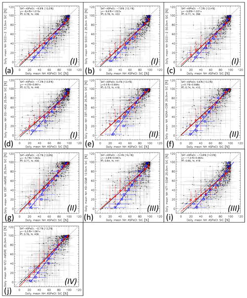
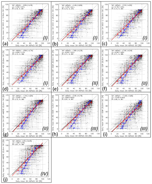
Figure 15 Scatterplots of co-located daily average SIC from visual ship-based observations (ASPeCt, x axis; note that these are Ice Watch/ASSIST for the Arctic) and the 10 satellite SIC algorithm products (SAT, y axes) for the Arctic during the years 2002–2011. Red symbols denote the average satellite SIC binned into 10 % ASPeCt SIC intervals (except 0 % … 5 % and 95 % … 100 %, where 5 % bins are used). Blue symbols denote the average ASPeCt SIC binned into 10 % satellite SIC intervals. Error bars denote 1 standard deviation of the average. Dotted lines denote the identity line. Solid lines denote the linear regression of the respective value pairs. The mean difference and the standard deviation, the linear regression equation, the number of valid data pairs (N), and the squared linear correlation coefficient (R²) are given in the top left of every image for the daily SIC values. Roman numbers I–IV denote the group assigned to the respective algorithm (see text for details).

Table 5 Summary of the statistics of the comparison between daily mean ship-based and satellite SIC data (see Fig. 15, black symbols) for – from top to bottom – the entire year, only winter and only summer. DIFF is the mean difference satellite minus ship-based SIC, and SD is the respective standard deviation; R² is the squared linear correlation coefficient. All concentration values are given in percent.

5.1 Arctic

Overall, for the Arctic, all 10 products compare reasonably well to the ship-based observations (Fig. 15, Table 5). At high concentrations ($>\sim$ 80 %), group I products and ASI–SSMI (Fig. 15a–d, h) exhibit the most symmetric distributions around the identity line. NT1–SSMI (Fig. 15i) shows an asymmetric distribution with a considerable fraction of satellite sea-ice concentrations even below 60 %, translating into a difference between satellite- and ship-based sea-ice concentrations of up to 40 %. Group II and IV products (Fig. 15e–g, j) show an asymmetric distribution with more high satellite-based than high ship-based sea-ice concentrations. Most products have more data pairs below the identity line; i.e. satellite-based are smaller than ship-based sea-ice concentrations as illustrated by a negative overall bias and regression lines located below the identity line for six of the 10 products (Table 5). Group II and IV products provide the smallest absolute overall bias of < 1 %. Biases are larger for group I, but at the same time the standard deviation of the difference (SD) is smallest for group I products. The highest correlations are obtained for CBT–AMSR-E and group I products, except OSI-450. We find the best linear fits, i.e. slopes closest to the identity line, however, for CBT–SSMI and NOAA CDR.

Figure 16 As Fig. 15 but for the Antarctic.

Table 6 As Table 5 but for the Antarctic (see Fig. 16, black symbols).

How do results of the entire year compare to those obtained separately for winter or summer months (see Fig. 5 for differences in the location of the ship-based observations)? For all products, the correlation is lower in winter than summer and the entire year. This can be explained by fewer observations during winter in general and by substantially fewer low sea-ice concentrations; most observations during winter are > 75 %. Except for ASI–SSMI, the differences in the bias between summer, winter, and the entire year are small (mostly < 1 %). All products except SICCI-12km and ASI–SSMI provide a lower SD in winter than summer. Compared to the other groups, group I exhibits the smallest SD in summer while group II does so in winter. OSI-450 stands out with the smallest inter-seasonal change in bias and SD of only ∼ 0.1 % (Table 5; see also Sect. 6.1.4).

We want to better visualize the average distribution of the two data sets and investigate the partitioning of the data into sea-ice concentration bins of 10 % width – the average accuracy of the ship-based sea-ice concentration observations. For this purpose we bin sea-ice concentrations of one data set, e.g. ship observations, into 10 % wide bins and compute the mean sea-ice concentration of the other data set (Fig. 15, red symbols) and vice versa (blue symbols). The binned values and associated regression lines illustrate even better the above-mentioned asymmetry in the distribution of the data pairs. For instance, NT1–SSMI (Fig. 15i) sea-ice concentration range between 60 % and 100 % over a ship-based observations range of 80 % to 100 %. Consequently, the average NT1–SSMI sea-ice concentration for the ship observation bin 95 %–100 % is ∼ 85 % (uppermost red triangle), while the average ship-based sea-ice concentration for the NT1–SSMI bin 95 %–100 % is ∼ 95 % (uppermost blue square). For two equally well-distributed data sets, one would expect that red and blue symbols and regression lines are close to each other. This is not the case and we refer to Sect. 6.1.4 for more discussion of this issue.

5.2 Antarctic

The scatterplots of the daily average along-track mean sea-ice concentrations for the Antarctic (Fig. 16) reveal, for sea-ice concentrations $>\sim$ 80 %, mostly symmetric distributions for seven of the 10 products. NT1–SSMI (Fig. 16i) has considerably more low than high sea-ice concentration values (compare Fig. 15i). NT2–AMSR-E (Fig. 16j) has almost no data points below the identity line at $>\sim$ 80 % with data pairs concentrated at 100 % satellite sea-ice concentration. A considerable drop in the count of data values above the identity line at lower concentrations results in a highly asymmetric distribution at concentrations below ∼ 50 %. Group II products have the lowest overall biases (Table 6) but slopes of the linear regression are considerably steeper than the identity line (Fig. 16e–g) in contrast to group III products (Fig. 16h, i) and OSI-450 (Fig. 16d). We find the largest bias for NT1–SSMI: −11.0 %. NT2–AMSR-E shows a considerable positive bias: +4.5 %. We find highest correlations between ship- and satellite-based observations for group I products and CBT–AMSR-E, the lowest SD values for group I products as well.

In contrast to the Arctic, correlations between ship- and satellite-based sea-ice concentrations are smaller in summer than winter when correlations are even higher than for the entire year for most products (Table 6). For all products, except group III, biases are smaller in winter than summer by mostly < 2 %. NT2–AMSR-E is the only product with a positive bias in both seasons. We find the largest inter-seasonal bias change for CBT–AMSR-E (2.7 %) and SICCI-25km (2.9 %) and the smallest for CBT–SSMI (0.4 %). For all products, the SD is smaller by 3 %–5 % (larger by 2 %–3 %) compared to the entire year in winter (in summer). Inter-seasonal SD changes are hence considerably larger in the Antarctic than in the Arctic (compare Tables 5 and 6).

Binning the sea-ice concentrations like described in Sect. 5.1 (red and blue symbols in Fig. 16) leads to the following main observations. (1) All products – except NT1–SSMI and NT2–AMSR-E – have the best agreement with ship-based observations in the sea-ice concentration range from 60 % to 80 %. (2) All products underestimate ship-based sea-ice concentrations for concentrations $<\sim$ 50 %. (3) The negative bias of ∼ 10 % observed for NT1–SSMI applies to the entire sea-ice concentration range. (4) NT2–AMSR-E is the only product overestimating ship-based sea-ice concentrations considerably; this overestimation reaches 10 % for the range 60 %–80 %. Apart from that, we find, like for the Arctic, that blue regression lines exhibit a considerably steeper slope than the red ones, suggesting that in the Antarctic the distribution of the data over the range 0–100 % is also asymmetric (see Sect. 6.1.4).

5.3 Summary and discussion of comparison against ship-based observations

Group II products provide the smallest overall difference from the ship-based observations: around 0 % (Arctic) and around −2 % (Antarctic). Group I products provide differences around −7.5 % (Arctic) and −3.5 % (Antarctic). Group I and II products share similar average correlations (R²) in the Arctic, 0.77 and 0.76, and in the Antarctic, 0.74 and 0.72. Standard deviations for group I products are smaller – by 1 % in the Arctic and by 2 % in the Antarctic – than for group II products. On average, these results are more accurate than those obtained for group III and IV products. We refrain from giving a ranking or recommendation as to which product is the best when compared to ship-based observations.

We find the lowest correlation for ASI–SSMI (group III) in both hemispheres. However, it is the product with the largest improvement in the inter-comparison results between winter and summer in the Arctic: correlation increases and difference and standard deviation decrease. This could be attributed to the higher fraction of intermediate sea-ice concentrations during summer for which the comparably fine grid resolution of 12.5 km of the ASI–SSMI product could be advantageous. There is evidence that this behaviour is coupled to the usage of the near-90 GHz channels because we observed a similar, albeit less pronounced, behaviour for SICCI-12km, which also employs near-90 GHz data and is provided at 12.5 km grid resolution (Table 2). Because in the Antarctic the sea-ice cover is more open year-round, it is plausible that we did not find similar behaviour there for these two products.

There are a few points to discuss. First of all, Figs. 15 and 16 reveal quite a high relative occurrence of sea-ice concentrations in the range from 95 % to 100 %. This might have biased our results. We therefore repeated our comparison by discarding all data pairs with daily mean sea-ice concentrations ≥ 95 %. The main results (not shown) are an overall increase in the differences by about 2 % and in the standard deviations by ∼ 1 % (group I) and 2 %–3 % (group II) and a reduction of the correlation by ∼ 0.08. Ranking between groups is otherwise not changed. Secondly, the results obtained for group I products are based on the truncated sea-ice concentrations. Using the non-truncated data does not considerably change our findings (not shown). Differences between satellite-based and ship-based sea-ice concentrations decrease by between 0 % and 0.3 % with a concomitant increase in the standard deviation of up to 0.2 %; this applies primarily to winter when the fraction of near-100 % sea-ice concentrations is large. Thirdly, application of the Gaussian fit method (see Sects. 2.1.4 and 6.1.3) seems inappropriate given the sea-ice concentration range considered in this inter-comparison. Even if it were, we can assume that differences and standard deviations obtained for the other products would change by less than 1 %. All these changes would be small compared to the accuracy of the ship-based sea-ice concentrations (see Sect. 2.3, beginning of Sects. 5, and 6.1.4).

In Figs. 15 and 16, several of the products exhibit points along the y=0 % sea-ice concentration line, i.e. conditions where sea ice is reported by the ship while the satellite estimates exactly 0 %. This applies mostly to group II products and ASI–SSMI (Fig. 15e–h). These points with zero daily mean sea-ice concentration are very likely the result of the weather filters applied (Sect. 2.1.3), which, in addition to removing false sea ice caused by atmospheric effects, also remove true sea ice (Ivanova et al., 2015; Lavergne et al., 2019). The combination of explicit atmospheric correction and dynamic tuning of the weather filter in group I products seems to reduce the occurrence of such cases notably (Figs. 15a–d; 16a–d).

6 Discussion and conclusions

6.1 Discussion

6.1.1 Observed differences in sea-ice area and extent

Time series of SIA and SIE have long been used to derive conclusions about the past development of the sea-ice cover and to even extrapolate its future development. In order to do so, such time series need to be sufficiently long, consistent and accurate. A long, consistent time series is typically obtained using a fundamental climate data record of brightness temperatures as input for the retrieval, as is done for group I product OSI-450, to ensure that inter-sensor differences are as small as possible. Our paper suggests that additional steps might be required, for instance dynamic retrieval of tie points and dynamic adaptation of weather filters (see Sect. 6.1.2), to reach the goal of a long-term consistent sea-ice concentration data set to be used to compute long-term consistent time series of SIA and SIE.

Meier and Steward (2019) suggested a method to obtain an estimate of SIE and NSIDC sea-ice index accuracy, which they found to be ∼ 50 000 km² under certain circumstances for the Arctic. They also pointed out, however, that there is a clear bias (or spread) of 500 000 km² to 1 million km² between SIE estimates from different products (see also Ivanova et al., 2014). Therefore, as long as one does not know which product provides the best representation of the actual sea-ice cover, one is left alone with a relatively precise estimate of the SIE, which might be biased, however, by an amount an order of magnitude larger. Notz (2014) found that the SIE and its trend provide a limited metric for the performance of numerical models. Petty et al. (2018) suggested that predictions of the September Arctic sea-ice minimum in area and extent would benefit from giving more weight to SIA. Niederdrenk and Notz (2018) concluded that observational uncertainty is the main source of uncertainty for estimating at which level of global warming the Arctic will lose its summer sea-ice cover. In the light of these findings, the inter-product differences in SIA and SIE resulting from our study provide useful information about which algorithm or group of algorithms is particularly well suited for investigations of SIA and SIE in just one hemisphere year-round or for an individual season. Because we were able to estimate the effect of the mismatch between true and grid resolution and of the interpolation across the observation gap around the North Pole and could further rule out influences of different land masks, we are confident that the inter-product differences observed mostly originate from differences in how the algorithms handle surface emissivity variations or variations in the atmospheric influence.

6.1.2 The role of weather filters

We illustrated that the weather filters implemented in each of the 10 products have quite different behaviour, despite the fact they all use the same gradient ratios of brightness temperature frequency channels. Potential users should be aware of this. We confirm that the dynamic open water filters designed for group I products (see Table 2) have a stable impact on the lower part of the sea-ice concentration, cutting through it at about 10 % SIC. This is across the months and changes of sensors (and thus frequencies, calibration, etc.) and for both hemispheres. We refer to Lavergne et al. (2019) for discussions about how this consistency could be improved further. The analysis also sheds light on how the other six products perform in terms of stability. Here, we are interested in both the temporal consistency of the weather filter effects (e.g. jumps across satellite series, across months, across climate-induced trends) and the absolute level at which they cut through the sea-ice concentration distribution, especially with respect to the 15 % threshold embedded in the SIE and SIA curves shown in Figs. 6 and 7. Group II products all cut around 15 %, sometimes below, sometimes above, but in general at a higher sea-ice concentration than group I products (Figs. 1 and 2). We observed evidence for an actual impact of weather filter cut-off sea-ice concentration variation over time in the SIE time series in winter in the Antarctic (Fig. 7c). We believe Figs. 1 and 2 are new illustrations that data products can differ in many ways. Such time series, adapted from Lavergne et al. (2019), are an effective tool for data producers and users to assess the temporal consistency of sea-ice concentration data products.

Table 7 Summary of hypothetic daily average sea-ice concentrations from Fig. 17 for the pack ice case (a) and the marginal ice zone (MIZ) (b). The left two columns show sea-ice concentrations as shown in Fig. 17; the middle two columns show the effect of sea-ice concentration underestimation for thin ice; and the right two columns show the effect of sea-ice concentration overestimation, e.g. thick ice with a wet snow cover (top), or of sea-ice concentration underestimation, e.g. MIZ during end of summer (bottom).

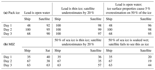
6.2 The impact of truncating sea-ice concentrations at 100 %

The analysis of the validation at 100 % conditions (Sect. 4) raises a critical question to be discussed in the future among data producers and with the data users: given that sea-ice concentration products are used following application of a 100 % sea-ice concentration threshold, is it better to have algorithms (slightly) overshoot the sea-ice concentration distribution or should data producers aim at an unbiased non-truncated distribution? To let algorithms overshoot will return fewer below-100 % estimates in the product files, which might be positive for large areas of the inner sea-ice cover during winter. However, one consequence of this (hypothetically) shifted sea-ice concentration distribution with modal values > 100 % is that the sea-ice concentration in areas with a true < 100 % sea ice concentration, i.e. 99 % or even 98 %, might be set to 100 %. Such areas could contain leads. According to Marcq and Weiss (2012) about 70 % of the upward ocean–atmosphere heat exchange occurs through leads, even though these cover only 1 % to 2 % of the central Arctic Ocean. Assuming a heat transfer through thick ice of 5 W m⁻² and through a lead of 400 W m⁻² (e.g. Marcq and Weiss, 2012, near-surface air temperature difference of 30 K) a heat flux calculation yields 5 W m⁻² for 100 % and ∼ 9 W m⁻² for 99 % true sea-ice concentration, an increase by 80 %. Using sea-ice concentrations of an algorithm with a modal value at 101 % or higher might therefore result in a substantial underestimation of the surface heat flux. Integrated over the sea-ice-covered central Arctic Ocean (area ∼ 7 million km²) this underestimation could be as high as 2.4×10¹² MJ d⁻¹.

To aim at an unbiased algorithm might help with a better sensitivity to small openings (but note the RMSE of non-truncated retrievals ranges between 2 % and 5 % for the various algorithms studied here); however, the product grid will have more below-100 % estimates. Our analysis, supported by the Gaussian fit method, introduces the question and opens the discussion, but does not provide an answer.

6.3 Observed differences to ship-based observations

One of the innovations of the products of group I (see Table 2) is the self-optimizing capability of the algorithms to adopt to seasonally changing sea-ice conditions, i.e. the transition between winter and summer. If ship-based sea-ice observations are as reliable in summer as they are in winter, then a comparison of the differences and standard deviations obtained in winter and summer could reveal how well an algorithm deals with the seasonally changing sea-ice conditions. If we focus on sea-ice concentrations < 95 % to avoid the clustering of data pairs near 100 % during winter, we find the CDRs of the group I products, SICCI-25km, SICCI-50km, and OSI-450, to stand out with winter-to-summer changes in the difference between ship- and satellite-based sea-ice concentrations around 0.2 %, compared to ∼ 3.5 % for group II products in the Arctic. Respective changes in the standard deviation range between 0.1 % and 5.2 % for group II but are near ∼ 2.7 % for group I CDRs. In the Antarctic, the smallest winter-to-summer differences of ∼ 0.3 % are obtained for group I products SICCI-12km and OSI-450, compared to ∼ 2.5 % for group II products. These provide a winter-to-summer change in standard deviation of ∼ 6.5 %, while SICCI-12km and OSI-450 exhibit values of ∼ 4.0 %. These results suggest that most group I products compare with the ship-based sea-ice observations more consistently across seasons than the other products.

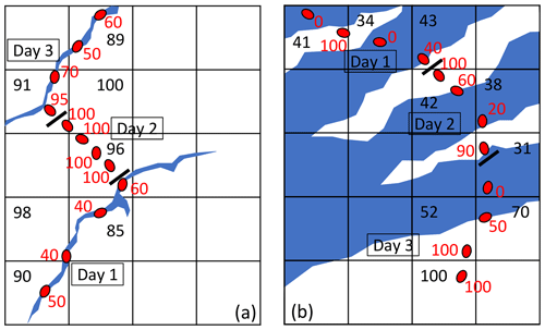
Figure 17 Illustration of the representativity of ship-based observations (red ellipses and numbers) compared to gridded satellite observations (black grid and numbers) for (a) close pack ice with leads and (b) an open sea-ice cover in the marginal ice zone. Size of ellipses is in scale with the grid cell size of 25 km by 25 km. Short black bars denote transitions between days. See also Table 7.

It is noteworthy, however, to keep in mind the difference in scales and observational limitations between ship-based and satellite-based observations of the sea-ice concentration – as illustrated in Fig. 17. For the pack ice–lead case (Fig. 17a, Table 7a), the variation in the ship-based observations depends strongly on the fraction of thin ice. For leads covered by open water, satellite sea-ice concentrations tend to exceed ship-based concentrations. This could explain the banana-shaped distribution of data pairs for the SH (Fig. 16). For leads covered by thin ice, it is the other way round. Ship observations would reveal a total sea-ice concentration of 100 %, while most of the tested algorithms underestimate the true sea-ice concentration in the presence of thin ice (Cavalieri, 1994; Comiso and Steffen, 2001; Ivanova et al., 2015). This could explain the larger fraction of ship-based sea-ice concentrations near 100 % as is particularly pronounced, e.g. for NT1–SSMI (Fig. 15i) and, in general, the larger range of satellite versus ship-based sea-ice concentrations at comparably high concentrations. For the marginal ice zone (Fig. 17b, Table 7b), it is more likely that most products provide smaller sea-ice concentrations than observed from a ship. During winter, a considerable fraction of the sea ice might be thin ice – causing underestimation as stated above. During summer, a considerable fraction of the sea ice might be too wet to be recognized as ice by satellite microwave radiometry – causing an underestimation as well (see e.g. Worby and Comiso, 2004; Ozsoy-Cicek et al., 2009). In addition, low ice concentrations are often filtered by the weather filters applied (see Sect. 2.1.3). This results in a substantially larger range of ship-based sea-ice concentrations at comparably low satellite sea-ice concentrations. Furthermore, this also results in a larger fraction of low ice concentration values for the satellite-based than the ship-based observations. This explains why mean ship-based sea-ice concentrations per binned satellite sea-ice concentration (blue symbols in Figs. 15 and 16) are shifted so much to the right compared to the red symbols; this is also evident from the larger fraction of data pairs below than above the identity line for sea-ice concentrations below 60 %–80 %.

We note that another data set of a different kind of ship-based observations of Arctic sea-ice conditions is available at the Arctic and Antarctic Research Institute (AARI) and has recently been used for a sea-ice concentration algorithm inter-comparison study using an approach different from the one used in our paper (Alekseeva et al., 2019). We might extend our inter-comparison studies to their data set in the future.

6.4 Conclusions

Recently, three new global sea-ice concentration (SIC) climate data records (CDRs) have been released. They are described in Lavergne et al. (2019). These products, SICCI-25km, SICCI-50km, and OSI-450, utilize a dynamic, self-optimizing hybrid sea-ice concentration algorithm, which is applied to satellite microwave brightness temperature measurements of the SMMR, SSM/I, and SSMIS instruments (OSI-450) or the AMSR-E and AMSR2 instruments (SICCI-25km and SICCI-50km); see Table 1 for instruments and frequencies. Within this paper, these new products are evaluated by means of an inter-comparison to seven other sea-ice concentration products (see Table 2 for acronyms, satellite sensors and frequencies used, and assignment to groups of algorithms I–IV) and with independent sea-ice cover data.

We find a very good and consistent agreement in inter-annual variation in the monthly mean SIA and SIE time series for both hemispheres for the overlap periods of the respective products used at their native grid resolution. We can explain unexpected low SIE of SICCI-50km during Arctic winter and Antarctic summer by the coarse resolution of the 6.9 GHz frequency observations combined with too aggressive filtering of near-coastal and potentially weather-influenced grid cells near coastlines, which removed a substantial number of grid cells with ice. We note that SIE differences are to be expected simply from the different grid resolutions. When inter-comparing products on the same grid (50 km) applying the same land mask, the products of group I provide quite similar values of SIC, SIA, and SIE for both hemispheres, during times of both maximum and minimum sea-ice cover. Overall differences are < 1.0 % for SIC and < 100 000 km² (Arctic) and < 200 000 km² (Antarctic) for both SIA and SIE. We find a similarly good agreement for the products CBT–SSMI and NOAA CDR of group II (see Table 2), as can be expected from the design of NOAA CDR (see Appendix F and Peng et al., 2013). We find the largest differences for NT1–SSMI and NT2–AMSR-E: NT1–SSMI provides less sea ice than other products, particularly in summer in the Arctic and winter in the Antarctic; NT2–AMSR-E provides more sea ice than other products in the Antarctic. Based on our results we state that it matters which algorithm and/or product is used for monitoring the polar sea-ice cover as long as one is interested in absolute values; similarity of trends has been shown elsewhere (e.g. Ivanova et al., 2014; Comiso et al., 2017a).

Results quoted in the previous paragraph rely on computations applying the often-used 15 % SIC threshold (e.g. Gloersen et al., 1992). Our investigations suggest that it might be worth starting to reconsider this threshold because, as illustrated in our paper, the weather filters applied might have inter-sensor jumps and fail to cut at a constant sea-ice concentration across the different satellite sensors used. For example, sea-ice concentrations from sensor A might be cut by the weather filter at 14 % while these might be cut at 17 % for a subsequent sensor B. As a result, more sea ice is removed for sensor B, and the sea-ice extent computed from sea-ice concentration data of sensor B is systematically smaller than that computed from sensor A. We observe evidence for this in our results. A more thorough analysis of trends over sub-periods observed by the 10 products could reveal other such impacts. This impact is likely to be particularly pronounced in the peripheral seas with a comparably large fraction of the marginal ice zone, such as the Bering Sea or the Barents Sea. Note that the OSI-450 algorithm provides a particularly stable weather-filter-induced sea-ice concentration cut-off at ∼ 10 % across the sensors used.

Sea-ice concentrations are retrieved from satellite microwave brightness temperatures using an empirical physical algorithm, which usually involves a limited set of tie points. However, the natural variability of surface properties relevant for microwave remote sensing of sea ice is large and these tie points can only be an average signature associated with a significant spread. As a result, sea-ice concentrations retrieved by such algorithms naturally vary around (below and above) 100 % even though the actual sea-ice concentration is exactly 100 %. The natural variability of the sea-ice surface properties and the linearity of most algorithms suggest that the spread of retrieved sea-ice concentrations around 100 % follows a Gaussian distribution. However, all 10 products examined here either truncate sea-ice concentrations at 100 %, i.e. fold retrieved values > 100 % to exactly 100 %, or do simply not allow retrieval of SIC > 100 % (NT2–AMSR-E) and the natural variability cannot be assessed. We develop a Gaussian fit method to reconstruct the full distribution of sea-ice concentrations around 100 %. We demonstrate its performance on the group I products (as these provide, for the first time, both the non-truncated and truncated values) and subsequently use it to reconstruct non-truncated sea-ice concentration distributions for the remaining six products (Fig. 3, and Appendix H, Figs. H1 and H2). Based on our results we conclude that it is worthwhile to rethink the concept of truncation at 100 % (but also at 0 % SIC) and critically reassess evaluation results at the two ends of the sea-ice concentration distribution. Indeed, we argue that direct evaluation of truncated data sets gives misleading information on the accuracy of the sea-ice concentration data and favours those data sets that overestimate sea-ice concentrations. Such overestimation has direct implications on the ability of a given sea-ice concentration data set to observe small openings in an otherwise complete sea-ice cover. We invite the sea-ice concentration data producers and users to take this into consideration and discuss the implications towards future versions of such data products.

Appendix A: The EUMETSAT OSI SAF–ESA CCI algorithm suite

The four products OSI-450, SICCI-12km, SICCI-25km, and SICCI-50km have in common that they are based on a hybrid, self-tuning, self-optimizing sea-ice concentration algorithm (Lavergne et al., 2019). This algorithm is applied to brightness temperature (TB) observations of the SMMR, SSM/I, and SSMIS instruments for OSI-450, providing a fully revised version of the OSI-409 CDR (Tonboe et al., 2016). This algorithm is applied to brightness temperatures measured by the AMSR-E and AMSR2 instruments for the SICCI CDRs. Apart from the input satellite data the processing chains are the same for these four products. The algorithm is a generalization of the Comiso bootstrap frequency mode algorithm (Appendix C) and of the Bristol algorithm (Smith and Barret, 1994; Smith 1996) and is described in detail in Lavergne et al. (2019). Two algorithms that each combine three frequency channels (e.g. ∼ 19 GHz at vertical polarization and ∼ 37 GHz at both horizontal and vertical polarizations) are respectively optimized to provide the best accuracy in open water (the B_OW algorithm) and consolidated ice (the B_CI algorithm) conditions. The sea-ice concentrations obtained with each of the two optimized algorithms are merged linearly into a hybrid sea-ice concentration SIC_hybrid according to the general formula

$$\begin{array}{}\text{(A1)}& \begin{array}{rl}& \left\{\begin{array}{ll}{w}_{\text{OW}}=\mathrm{1};& \mathrm{for}{B}_{\text{OW}}<\mathrm{0.7}\\ w_{\text{OW}}=\mathrm{0};& \mathrm{for}{B}_{\text{OW}}>\mathrm{0.9}\\ w_{\text{OW}}=\mathrm{1}-\frac{B_{\text{OW}}-\mathrm{0.7}}{\mathrm{0.2}};& \mathrm{for}{B}_{\text{OW}}\in [\mathrm{0.7};\mathrm{0.9}]\end{array}\right.;\\ & {\text{SIC}}_{\text{hybrid}}=w_{\text{OW}}\times B_{\text{OW}}+(\mathrm{1}-w_{\text{OW}})\times B_{\text{CI}}.\end{array}\end{array}$$

For sea-ice concentrations below 70 %, SIC_hybrid relies completely on B_OW and for sea-ice concentrations above 90 % it relies entirely on B_CI. The B_OW and B_CI algorithms can be regarded as a generalized version of the Comiso bootstrap and Bristol algorithms, in the sense that they combine the three different brightness temperature channels used by the two algorithms in a three-dimensional TB space and optimize their data projection plane for the best accuracy.

In this paper, we use the sea-ice concentration CDR derived from SMMR, SSM/I, and SSMIS data: OSI-450 (https://doi.org/10.15770/EUM_SAF_OSI_0008, OSI SAF, 2017) and two sea-ice concentration CDRs derived from AMSR-E and AMSR2 data: SICCI-25km (https://doi.org/10.5285/f17f146a31b14dfd960cde0874236ee5, Pedersen et al., 2017a) and SICCI-50km (https://doi.org/10.5285/5f75fcb0c58740d99b07953797bc041e, Pedersen et al., 2017b).

While SICCI-25km is based on brightness temperatures measured at ∼ 19 and ∼ 37 GHz, similar to OSI-450, SICCI-50km is based on brightness temperatures measured at ∼ 7 and ∼ 37 GHz. OSI-450 and SICCI-25km come at 25 km grid resolution while SICCI-50km has 50 km grid resolution. In addition, we use a fourth product, SICCI-12km, which is provided at 12.5 km grid resolution and is based on brightness temperatures measured by AMSR-E and AMSR2 at ∼ 19 and ∼ 90 GHz. Here, we use a prototype of SICCI-12km, which was produced during the ESA CCI Sea Ice project, but was not released publicly (partly based on the results presented in this paper). All these data sets have daily temporal resolution and are provided on polar EASE-Grid version 2.0 (Brodzik et al., 2012, 2014).

Appendix B: The ARTIST sea-ice (ASI) algorithm

The ARTIST Sea Ice (ASI) algorithm (Kaleschke et al., 2001; Spreen et al., 2008) is a modified hybrid of the near-90 GHz algorithm (Svendsen et al., 1987) and the NASA Team algorithm (see Appendix D). Water and ice are distinguished at high resolution by the TB polarization difference (P) at ∼ 90 GHz:

$$P={\text{TB}}_{\mathrm{90}}^{\text{V}}-{\text{TB}}_{\mathrm{90}}^{\text{H}}.$$

The basic equations for the ASI algorithm are based on the near-90 GHz algorithm of Svendsen et al. (1987):

$$\begin{array}{}\text{(B1)}& P=a\times \left(C\times \mathrm{\Delta }{\mathit{ϵ}}_{\text{ice}}\times T_{\text{ice}}+(\mathrm{1}-C)\times \mathrm{\Delta }{\mathit{ϵ}}_{\text{water}}\times T_{\text{water}}\right),\end{array}$$

with the atmospheric influence $a=(\mathrm{1.1}\times e^{-\mathit{\tau }}-\mathrm{0.11})\times e^{-\mathit{\tau }}$; C is the total sea-ice concentration, T is the temperature, Δϵ is the difference in surface emissivity between vertical and horizontal polarization for the ice or water surface fraction, and τ is the total atmospheric optical depth for Arctic conditions at this frequency and viewing conditions. For ice-free (C=0) and totally ice-covered (C=1) conditions, Eq. (B1) yields the tie points for open water $P_{\text{water}}=a_{\text{water}}\times \mathrm{\Delta }{\mathit{ϵ}}_{\text{water}}\times T_{\text{water}}$ and sea ice $P_{\text{ice}}=a_{\text{ice}}\times \mathrm{\Delta }{\mathit{ϵ}}_{\text{ice}}\times T_{\text{ice}}$. Taylor expansions of Eq. (B1) around C=0 and C=1 lead to a pair of equations for P, in which the atmospheric influences a_water and a_ice can be substituted with the aid of the tie point equations – provided that the variation in the atmospheric influence is small over water or ice (see Spreen et al., 2008). After substitution one obtains

$$\begin{array}{}\text{(B2)}& {\displaystyle }\begin{array}{rl}& C=\left({\displaystyle \frac{P}{P_{\text{water}}}}-\mathrm{1}\right)\times \left({\displaystyle \frac{\mathrm{\Delta }{\mathit{ϵ}}_{\text{water}}\times T_{\text{water}}}{\mathrm{\Delta }{\mathit{ϵ}}_{\text{ice}}\times T_{\text{ice}}-\mathrm{\Delta }{\mathit{ϵ}}_{\text{water}}\times T_{\text{water}}}}\right)\\ & \text{for}C\to \mathrm{0},\end{array}\text{(B3)}& {\displaystyle }\begin{array}{rl}& C={\displaystyle \frac{P}{P_{\text{ice}}}}+\left({\displaystyle \frac{P}{P_{\text{ice}}}}-\mathrm{1}\right)\times \left({\displaystyle \frac{\mathrm{\Delta }{\mathit{ϵ}}_{\text{water}}\times T_{\text{water}}}{\mathrm{\Delta }{\mathit{ϵ}}_{\text{ice}}\times T_{\text{ice}}-\mathrm{\Delta }{\mathit{ϵ}}_{\text{water}}\times T_{\text{water}}}}\right)\\ & \text{for}C\to \mathrm{1}.\end{array}\end{array}$$

According to Svendsen et al. (1987) the ratio of the surface emissivity differences can be set to a constant value (−1.14). With this simplification and by assuming that the atmospheric influence inherent in P is a smooth function of the sea-ice concentration, one can use a 3rd-order polynomial function to interpolate between the solutions of Eqs. (B2) and (B3) to obtain sea-ice concentrations between 0 and 1 as a function of P:

$$\begin{array}{}\text{(B4)}& C\left(P\right)=d_{\mathrm{3}}\times P^{\mathrm{3}}+d_{\mathrm{2}}\times P^{\mathrm{2}}+d_{\mathrm{1}}\times P+d_{\mathrm{0}}.\end{array}$$

The coefficients d_i are derived with a linear equation system based on Eqs. (B2) and (B3) and their first derivatives (Spreen et al., 2008).

The larger, compared to the lower frequencies used in most products (see Table 2), weather influence at ∼ 90 GHz frequencies by atmospheric water content and surface wind speed can cause substantial overestimation of the sea-ice concentration over open water and within the ice edge (Kern, 2004; Andersen et al., 2006). Over open water, the weather influence is reduced by combining sea-ice concentrations obtained with Eq. (B4) with the NASA Team algorithm (NTA; see also Appendix D) sea-ice concentrations following

$$\begin{array}{}\text{(B5)}& \begin{array}{rl}& C=C_{\text{ASI}}\text{for}{C}_{\text{NTA}}>\mathrm{5}\mathit{\%},\\ & C=\mathrm{0}\mathit{\%}\text{for}{C}_{\text{NTA}}\le \mathrm{5}\mathit{\%}.\end{array}\end{array}$$

Hence, the ASI algorithm is a hybrid of the near-90GHz algorithm (Eqs. B1–B4) and the NTA (Kaleschke et al., 2001; Ezraty et al., 2007; Fanny Girard-Ardhuin, IFREMER, Brest, France, personal communication, 3 June 2019).

We use the ASI algorithm sea-ice concentration product provided via the Integrated Climate Data Center: https://icdc.cen.uni-hamburg.de (last access date: 27 February 2019). This product is processed at the French Institute for Exploitation of the Sea (IFREMER) from SSM/I and SSMIS data and provided via ICDC after application of a running 5 d median filter, further reducing spurious weather-influenced sea-ice concentration in the open water (Kern et al., 2010), on a polar-stereographic grid with 12.5 km grid resolution (at 70^∘ latitude). We abbreviate these data as ASI–SSMI.

Appendix C: The Comiso bootstrap algorithm

The Comiso bootstrap algorithm (Comiso, 1986; Comiso et al., 1997, 2003; Comiso and Nishio, 2008) combines TB observations at either two different frequencies (frequency mode, 37 and 19 GHz, vertical polarization) or at two different polarizations (polarization mode, 37 GHz, vertical and horizontal polarization). It is based on the observation that brightness temperatures measured at these frequencies/polarizations over closed sea ice tend to cluster along a line (ice line) while those over open water tend to cluster around a single point in the respective two-dimensional brightness temperature space. The total sea-ice concentration is computed using

$$\begin{array}{}\text{(C1)}& C={\displaystyle \frac{{\text{TB}}_f^{\text{V}}-{\text{TB}}_{f,\text{OW}}^{\text{V}}}{{\text{TB}}_{f,I}^{\text{P}}-{\text{TB}}_{f,\text{OW}}^{\text{V}}}},\end{array}$$

with the brightness temperature measured at vertical polarization and frequency f=37 GHz (polarization mode) or f=19 GHz (frequency mode): ${\text{TB}}_f^{\text{V}}$, the open water tie point ${\text{TB}}_{f,\text{OW}}^{\text{V}}$ at vertical polarization and the same frequency as ${\text{TB}}_f^{\text{V}}$ and the intersection of the ice line with a line from the open water tie point through the observed brightness temperature: ${\text{TB}}_{f,I}^{\text{P}}=A\times \frac{B-W}{Q-A}+B$. Scalars A and B are functions of the ice tie points for first-year ice (FYI) and multiyear ice (MYI) at 37 GHz at vertical and horizontal polarization (polarization mode) or at 19 and 37 GHz, both with vertical polarization (frequency mode). Q and W are functions of the actually observed brightness temperature and the water tie point at the respective frequencies and polarizations. The two algorithms (frequency and polarization mode) are combined so that only the polarization mode is used in high-concentration conditions, and otherwise the frequency mode is used.

We use daily gridded sea-ice concentrations derived with the Comiso bootstrap (CBT) algorithm from SMMR, SSM/I, and SSMIS instruments, as processed at NASA Goddard Space Flight Center (GSFC) and made available at https://nsidc.org/data/nsidc-0079 (last access: 7 February 2019). They are on a polar-stereographic grid with 25 km grid resolution (at 70^∘ latitude). We abbreviate these data as CBT–SSMI. For practical reasons, we access these GSFC CBT–SSMI fields from the NOAA sea-ice concentration CDR (Appendix F) files, where they are provided as additional data (Meier and Windnagel, 2018). The GSFC CBT–SSMI sea-ice concentration data set involves manual filtering, especially at the beginning of the record (SMMR period).

In addition, we use daily gridded sea-ice concentrations derived with this algorithm from AMSR-E data (Comiso et al., 2003; Comiso and Nishio, 2008) as provided by NSIDC (AE_SI25.003, Cavalieri et al., 2014, https://nsidc.org/data/ae_si25/versions/3, last access date: 26 April 2018) on the same polar-stereographic grid. The AMSR-E Comiso bootstrap algorithm sea-ice concentration is referred to as CBT–AMSR-E throughout this paper. Note that the NSIDC product AE_SI25.003 does not contain CBT–AMSR-E sea-ice concentrations itself. It contains the NT2 sea-ice concentration and the difference “Comiso bootstrap minus NT2 sea-ice concentration”. Therefore, we needed to compute the CBT–AMSR-E sea-ice concentration by adding the NT2 sea-ice concentration to that difference.

Appendix D: The NASA Team algorithm

The NASA Team algorithm (Cavalieri et al., 1984, 1992, 1999) combines the large difference of the normalized brightness temperature polarization difference at 19 GHz, $\text{PR}=\frac{{\text{TB}}_{\mathrm{19}}^{\text{V}}-{\text{TB}}_{\mathrm{19}}^{\text{H}}}{{\text{TB}}_{\mathrm{19}}^{\text{V}}+{\text{TB}}_{\mathrm{19}}^{\text{H}}}$, between water and ice, with the observation that the normalized brightness temperature frequency difference between 37 and 19 GHz at vertical polarization, $\text{GR}=\frac{{\text{TB}}_{\mathrm{37}}^{\text{V}}-{\text{TB}}_{\mathrm{19}}^{\text{V}}}{{\text{TB}}_{\mathrm{37}}^{\text{V}}+{\text{TB}}_{\mathrm{19}}^{\text{V}}}$, is negative for MYI and close to zero or slightly positive for FYI and open water. The total sea-ice concentration is derived as the sum of the fractions of MYI and FYI, which is constrained to a maximum of 1:

$$\begin{array}{}\text{(D1)}& \begin{array}{rl}& C_{\text{FYI}}={\displaystyle \frac{F_{\mathrm{0}}+F_{\mathrm{1}}\times \text{PR}+F_{\mathrm{2}}\times \text{GR}+F_{\mathrm{3}}\times \text{PR}\times \text{GR}}{D}},\\ & C_{\text{MYI}}={\displaystyle \frac{M_{\mathrm{0}}+M_{\mathrm{1}}\times \text{PR}+M_{\mathrm{2}}\times \text{GR}+M_{\mathrm{3}}\times \text{PR}\times \text{GR}}{D}},\\ & \text{with}D=D_{\mathrm{0}}+D_{\mathrm{1}}\times \text{PR}+D_{\mathrm{2}}\times \text{GR}+D_{\mathrm{3}}\times \text{PR}\times \text{GR},\end{array}\end{array}$$

where coefficients F_i, M_i, and D_i include the tie point information.

We use daily gridded sea-ice concentrations derived with the NASA Team (NT1) algorithm from SMMR, SSM/I, and SSMIS instruments, as processed at NASA Goddard Space Flight Center (GSFC), and made available at https://nsidc.org/data/nsidc-0051 (last access: 7 February 2019). They are on a polar-stereographic grid with 25 km grid resolution (at 70^∘ latitude). We abbreviate these data as NT1–SSMI. For practical reasons, we access these GSFC NT1–SSMI fields from the NOAA sea-ice concentration CDR (Appendix F) files, where they are provided as additional data (Meier et al., 2017; Meier and Windnagel, 2018). The GSFC NT1–SSMI sea-ice concentration data set involves manual filtering, especially at the beginning of the record (SMMR period).

Appendix E: The enhanced NASA Team algorithm (NT2)

Inter-comparison studies such as those of Comiso and Steffen (2001) and Comiso et al. (1997) led to the development of the enhanced NASA Team algorithm (NT2) (Markus and Cavalieri, 2000; Comiso et al., 2003) to mitigate effects such as layering in snow on sea ice on the accuracy of the sea-ice concentrations obtained with NT1. NT2 is conceptually different from the other algorithms presented here. The three relevant parameters (see below) are modelled as a function of sea-ice concentration in steps of 1 % for 12 different atmospheric states using a radiative transfer model. The sea-ice concentration resulting in the minimum cost function between modelled and observed values of these parameters is taken as the retrieved total sea-ice concentration. The three parameters used are selected such that the influence of layering in snow on sea ice is mitigated.

$$\begin{array}{}\text{(E1)}& \begin{array}{rl}& \mathrm{\Delta }\text{GR}={\displaystyle \frac{{\text{TB}}_{\mathrm{90}}^{\text{H}}-{\text{TB}}_{\mathrm{19}}^{\text{H}}}{{\text{TB}}_{\mathrm{90}}^{\text{H}}+{\text{TB}}_{\mathrm{19}}^{\text{H}}}}-{\displaystyle \frac{{\text{TB}}_{\mathrm{90}}^{\text{V}}-{\text{TB}}_{\mathrm{19}}^{\text{V}}}{{\text{TB}}_{\mathrm{90}}^{\text{V}}+{\text{TB}}_{\mathrm{19}}^{\text{V}}}}\\ & {\text{PR}}_{\mathrm{19}}^{\text{rotated}}=-{\displaystyle \frac{{\text{TB}}_{\mathrm{37}}^{\text{V}}-{\text{TB}}_{\mathrm{19}}^{\text{V}}}{{\text{TB}}_{\mathrm{37}}^{\text{V}}+{\text{TB}}_{\mathrm{19}}^{\text{V}}}}\\ & \times \sin {\mathit{\theta }}_{\mathrm{19}}+{\displaystyle \frac{{\text{TB}}_{\mathrm{19}}^{\text{V}}-{\text{TB}}_{\mathrm{19}}^{\text{H}}}{{\text{TB}}_{\mathrm{19}}^{\text{V}}+{\text{TB}}_{\mathrm{19}}^{\text{H}}}}\times \cos {\mathit{\theta }}_{\mathrm{19}}\\ & {\text{PR}}_{\mathrm{90}}^{\text{rotated}}=-{\displaystyle \frac{{\text{TB}}_{\mathrm{37}}^{\text{V}}-{\text{TB}}_{\mathrm{19}}^{\text{V}}}{{\text{TB}}_{\mathrm{37}}^{\text{V}}+{\text{TB}}_{\mathrm{19}}^{\text{V}}}}\\ & \times \sin {\mathit{\theta }}_{\mathrm{90}}+{\displaystyle \frac{{\text{TB}}_{\mathrm{90}}^{\text{V}}-{\text{TB}}_{\mathrm{90}}^{\text{H}}}{{\text{TB}}_{\mathrm{90}}^{\text{V}}+{\text{TB}}_{\mathrm{90}}^{\text{H}}}}\times \cos {\mathit{\theta }}_{\mathrm{90}}\end{array}\end{array}$$

The rotation is done in the space given by PR₁₉ and GR (see Appendix D) or by PR₉₀ and GR for ${\text{PR}}_{\mathrm{19}}^{\text{rotated}}$ and ${\text{PR}}_{\mathrm{90}}^{\text{rotated}}$, respectively, at an angle Θ chosen such that the ice lines in the respective space are parallel to the GR axis.

We use daily gridded NT2 sea-ice concentrations derived from AMSR-E data as provided by NSIDC: AE_SI25.003 (Cavalieri et al., 2014, https://nsidc.org/data/ae_si25/versions/3, last access date: 26 April 2018) on a polar-stereographic grid with 25 km grid resolution. We abbreviate these data as NT2–AMSR-E.

Appendix F: The NOAA NSIDC sea-ice concentration CDR

The NOAA NSIDC sea-ice concentration CDR combines sea-ice concentrations computed with the NT1 algorithm (Appendix D) with those computed with the CBT algorithm (Appendix C), via

$$\begin{array}{}\text{(F1)}& C=\left(C_{\text{NT1}},C_{\text{CBT}}\right)\end{array}$$

within the ice edge. The ice edge is defined by the CBT sea-ice concentration of 10 %. The generation and characteristics of the NOAA NSIDC CDR as well as details about filters (see also Sect. 2.1) and about the statistical uncertainty estimate provided with the product are described in Peng et al. (2013) and Meier and Windnagel (2018). We use the daily gridded sea-ice concentration data of NOAA NSIDC CDR version 3, named NOAA CDR in this paper, provided by NSIDC on a polar-stereographic grid with 25 km grid resolution (Meier et al., 2017, https://nsidc.org/data/g02202/versions/3, last access date: 7 February 2019).

It is important to note that the data sets NT1–SSMI (Appendix D) and CBT–SSMI (Appendix C), both from GSFC, are not used as input in the NOAA NSIDC CDR. Instead, sea-ice concentrations are computed at NSIDC using re-implementations of the two algorithms, which allow for a fully automated and transparent processing as required for a CDR, and combined with Eq. (F1). One of the key differences between the NSIDC and GSFC versions is that the NSIDC ones do not involve manual editing and start with SSM/I in July 1987.

Appendix G: Matrices of sea-ice concentration, area, and extent differences

This subsection contains the full set of matrices of differences between all 10 products of the overall hemispheric average monthly mean sea-ice concentration of the AMSR-E measurement period and of the respective overall monthly mean sea-ice area (SIA) and extent (SIE) in Figs. G1–G6.

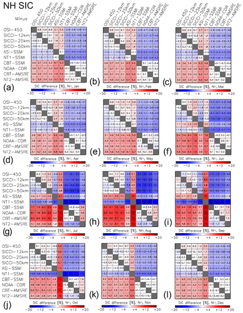
Figure G1 Differences between all 10 products of the average sea-ice concentration for the Arctic. The averages are computed from monthly mean values of the respective months of the AMSR-E period June 2002 to September 2011. All data are on the EASE-Grid 2.0 with 50 km grid resolution. The land mask of the SICCI-50km product is applied to all products.

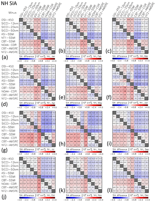
Figure G2 Differences between all 10 products of the average sea-ice area (SIA) for the Arctic. The differences are computed from monthly mean SIA of the respective months of the AMSR-E period June 2002 to September 2011. All data are on the EASE-Grid 2.0 with 50 km grid resolution. The land mask of the SICCI-50km product is applied to all products.

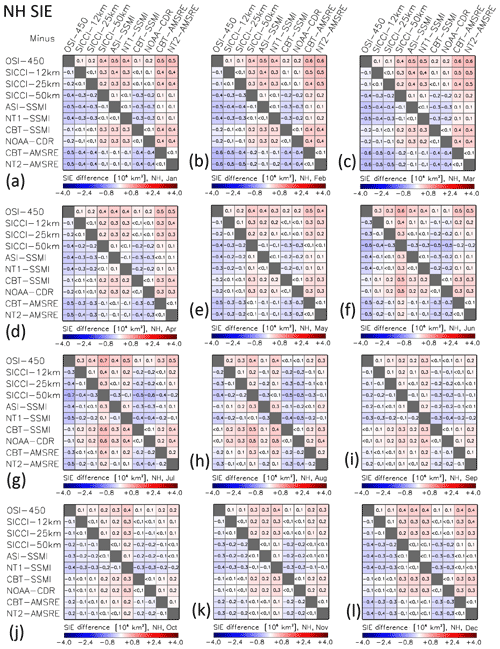
Figure G3 Differences between all 10 products of the average sea-ice extent (SIE) for the Arctic. The differences are computed from monthly mean SIE of the respective months of the AMSR-E period June 2002 to September 2011. All data are on the EASE-Grid 2.0 with 50 km grid resolution. The land mask of the SICCI-50km product is applied to all products.

Figure G4 As Fig. G1 but for the Antarctic.

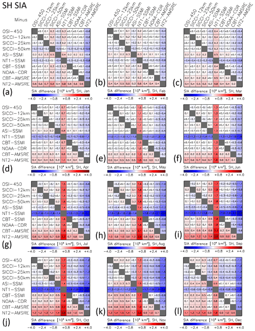
Figure G5 As Fig. G2 but for the Antarctic. Note the larger range of the SIA differences compared to the Arctic.

Figure G6 As Fig. G3 but for the Antarctic. Note the larger range of the SIE differences compared to the Arctic.

Appendix H: Gaussian fits for all 10 products

This subsection contains the two sets of Gaussian fits obtained for the Arctic (Fig. H1) and Antarctic (Fig. H2) based on the methodology described in Sect. 2.1.4; see also Fig. 3). These are the fits obtained from data of the overlap period between the AMSR-E measurement period and the RRDP2 near-100 % reference sea-ice concentration data set period, that is in winter of the years 2007–2011.

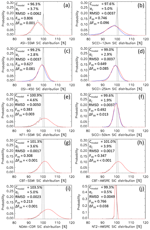
Figure H1 Sea-ice concentration distribution at RRDP2 near-100 % reference sea-ice concentration locations in the Arctic during winter for 2007–2011. Black symbols and lines show values cut off at 100 %; blue lines denote the original distribution (for OSI-450, SICCI-12km, SICCI-25km, and SICCI-50km); red lines denote the distribution resulting from the Gaussian fit to values of the distribution ≤ 99 %. In each image the modal sea-ice concentration (centre of the Gaussian fit: C_modal), the standard deviation of the fit σ_C and fit parameters with respect to the fraction of the distribution ≤ 99 % (F₉₉, ΔF₉₉; see text in Sect. 2.1.4 for a more detailed explanation), and the root-mean-squared difference (RMSD) between original and fitted probability are given.

Figure H2 As Fig. H1 but for the Antarctic.