Differential interferometric synthetic aperture radar for tide modelling in Antarctic ice-shelf grounding zones

Differential interferometric synthetic aperture radar (DInSAR) is an essential tool for detecting ice-sheet motion near Antarctica's oceanic margin. These space-borne measurements have been used extensively in the past to map the location and retreat of ice-shelf grounding lines as an indicator for the onset of marine ice-sheet instability and to calculate the mass balance of ice sheets and individual catchments. The main difficulty in interpreting DInSAR is that images originate from a combination of several SAR images and do not indicate instantaneous ice deflection at the times of satellite data acquisitions. Here, we combine the sub-centimetre accuracy and spatial benefits of DInSAR with the temporal benefits of tide models to infer the spatio-temporal dynamics of ice–ocean interaction during the times of satellite overpasses. We demonstrate the potential of this synergy with TerraSAR-X data from the almost-stagnant southern McMurdo Ice Shelf (SMIS). We then validate our algorithm with GPS data from the fast-flowing Darwin Glacier, draining the Antarctic Plateau through the Transantarctic Mountains into the Ross Sea. We are able to reconstruct DInSAR-derived vertical displacements to 7 mm mean absolute residual error and generally improve traditional tide-model output by up to 39 % from 10.8 to 6.7 cm RMSE against GPS data from areas where ice is in local hydrostatic equilibrium with the ocean and by up to 74 % from 21.4 to 5.6 cm RMSE against GPS data in feature-rich coastal areas where tide models have not been applicable before. Numerical modelling then reveals Young's modulus of $E=\mathrm{1.0}\pm \mathrm{0.56}$ GPa and an ice viscosity of $\mathit{\nu }=\mathrm{10}\pm \mathrm{3.65}$ TPa s when finite-element simulations of tidal flexure are matched to 16 d of tiltmeter data, supporting the hypothesis that strain-dependent anisotropy may significantly decrease effective viscosity compared to isotropic polycrystalline ice on large spatial scales. Applications of our method include the following: refining coarsely gridded tide models to resolve small-scale features at the spatial resolution and vertical accuracy of SAR imagery, separating elastic and viscoelastic contributions in the satellite-derived flexure measurement, and gaining information about large-scale ice heterogeneity in Antarctic ice-shelf grounding zones, the missing key to improving current ice-sheet flow models. The reconstruction of the individual components forming DInSAR images has the potential to become a standard remote-sensing method in polar tide modelling. Unlocking the algorithm's full potential to answer multi-disciplinary research questions is desired and demands collaboration within the scientific community.

1 Introduction

The periodic rise and fall of the ocean's surface is caused by the gravitational interplay of the Earth–Moon–Sun system and our planet's rotation. Knowledge of ocean tides is fundamental to fully understanding oceanic processes, sedimentation rates and behaviour of marine ecosystems. In Antarctica, the tidal oscillation also controls the motion of ice sheets near the coastline and ocean mixing in the sub-ice-shelf cavity, which modifies heat transport to the ice–ocean interface (Padman et al., 2018).

Synthetic aperture radar (SAR) satellites repeatedly illuminate Earth's surface and record the backscattered radar wave. While the SAR signal's amplitude depends on reflection intensity and is mainly characterised by physical and electrical properties of the surface, the recorded phase holds information about the distance travelled by the signal (Massom and Lubin, 2006). Two-pass interferometry (InSAR) can be used to determine surface motion with sub-centimetre accuracy over vast remote areas. Therefore, InSAR has been applied to measure Antarctic-wide ice velocity (Mouginot et al., 2019) and to observe tidal strain of landfast sea ice (Han and Lee, 2018). In grounding-zone areas, where an ice sheet comes into contact with the ocean for the first time and forms floating glaciers and ice shelves, InSAR has become the state-of-the-art practice for measuring the flux divergence of ice-flow velocity (Mouginot et al., 2014; Han and Lee, 2015) and thus the mass balance of many ice shelves around Antarctica (Rignot et al., 2013). InSAR can also be used to identify vertical deflection due to ocean tides. Horizontal and vertical motion cannot be distinguished in single interferograms, but the unsteady tidal contribution can be extracted by using triple or quadruple combinations of SAR images. This is based on the assumption that horizontal flow is time-invariant and that its phase contribution therefore cancels out. The double-differential measurement of vertical displacement only is known as differential interferometric synthetic aperture radar (DInSAR). While DInSAR has often been applied to detect the grounding-line movement around Antarctica (Konrad et al., 2018) the signal can also be used to measure spatial variability in ocean tides at very high ground resolution (Minchew et al., 2017; Baek and Shum, 2011). This second application is complicated by the fact that DInSAR interferograms show a combination of multiple stages of the tidal oscillation. Tidal migration of the grounding line as well as viscoelastic time delays in ice displacement, tidally induced velocity variations and geometric effects on the surface flexure also complicate the correct interpretation of DInSAR interferograms to date (Rack et al., 2017; Wild et al., 2018).

Present-day displacement measurements by interferometry are exacerbated by the requirement of phase unwrapping, which is the most crucial processing step in any InSAR method. Discontinuities in the fringe pattern can cause jumps in the unwrapped phase and may therefore bias the continuous motion field. Due to these complications, only very few studies have attempted to derive a tide model from DInSAR. Minchew et al. (2017) developed an unprecedented spatially and temporally dense SAR data acquisition campaign for the Rutford Ice Stream, Weddell Sea. Their novel Bayesian method to unequivocally separate a complete set of tidal harmonics from nontidal ice-surface variability is unique but beyond the sparse data availability for the remainder of Antarctica. Baek and Shum (2011) succeeded in using data from the ERS-1 and ERS-2 tandem mission to map the dominant tidal constituent (O₁) in Sulzberger Bay, Ross Sea, but data limitations prevented them from developing a full tidal model. In this case, too short a time span (71 d) of the ERS tandem mission eliminated a sufficient change of the observed tidal amplitudes, as aliasing problems between the repeat-pass cycle of the SAR satellites and the tidal oscillation masked the sensor's sensitivity to tidal variability. As a result, many tidal constituents had their variability too poorly sampled to derive a full set of tidal harmonics. However, even identifying only dominant single tidal constituents is valuable, as it indicates ways in which tide models need to be changed, and these changes will ultimately improve modelling of other constituents. In the Ross Sea, the tidal oscillation is dominated by diurnal harmonics (Padman et al., 2018).

Tide models can be consulted to predict both the timing and magnitude of the dominant harmonics. Numerous tide models of various spatial scales (global vs regional) and complexity have been developed (see Stammer et al., 2014, for an overview). While forward models integrate the equations of fluid motion subjected to a gravitational forcing over time, inverse models assimilate measurements of vertical displacement from laser altimetry, tide gauges and GPS (Egbert and Erofeeva, 2002; Padman et al., 2003a, 2008). Since the modelled physics is generally simple and gravitational forces are well known, tide-model predictions are of high quality in areas where ice is freely floating on the ocean. In coastal areas, tide models are prone to inaccuracies due to errors in model bathymetry, grounding-line location and insufficient knowledge of the ice water drag coefficient (Padman et al., 2018). Another source of error arises from the conversion of ice-shelf draft to ice-shelf thickness and subsequent estimation of water-column thickness. This freeboard conversion assumes that ice near the coastline is in local hydrostatic equilibrium, whereas stresses from the grounded ice clearly prevent a freely floating state. A bias of the hydrostatic solution towards thicker ice (Marsh et al., 2014), and therefore a thinning water-column thickness, may negatively affect the tidal prediction. In summary, the relatively coarse spatial resolution and underlying assumptions of contemporary tide models introduce inaccuracies especially in feature-rich coastal areas such as fjord-type outlet glaciers. Although average tide-model accuracy has improved markedly in coastal areas over 1 decade, from about ±10 cm (Padman et al., 2002) to ±6.5 cm (Stammer et al., 2014), it is still an order of magnitude larger than the sub-centimetre accuracy of DInSAR (Rignot et al., 2011). For this reason, we consider DInSAR to be the absolute truth and use these space-borne measurements to correct tide-model output.

In this paper, we show how the spatial benefits and high accuracy of DInSAR can be used to refine coarse-resolution tide models to adequately resolve ocean tides along the feature-rich Antarctic coastline. First we introduce the necessary dataset and describe the preprocessing. Second we test the algorithm for the southern McMurdo Ice Shelf (SMIS), a small and almost-stagnant ice shelf with a simple grounding-zone geometry, and expand the study to the Darwin Glacier, a relatively fast-flowing outlet glacier within a complex fjord-like embayment. We validate our results with dedicated field measurements taken within the Transantarctic Ice Deflection Experiment (TIDEx) in 2016. We then demonstrate how this exercise can also be applied to reveal errors in interferometric phase unwrapping and answer fundamental questions about the physical properties of ice in Antarctic glaciology.

2 Methodology

2.1 Summary of SAR image processing

To develop the method, we use 11 d repeat-pass TerraSAR-X data in StripMap imaging mode. The satellite acquires X-band radar data (wavelength 3.1 cm, frequency 9.6 GHz) with a ground resolution of slightly below 3 km×3 km and images covering an area of 30 km×50 km in look and azimuth direction. We calculate vertical surface displacement due to ocean tides using the GAMMA software package (Werner et al., 2000). InSAR and DInSAR image combinations are generally chosen so that a later image is always subtracted from an earlier image. For image triplets, the central SAR image serves as a common reference during the co-registration. We then correct the resulting DInSAR interferograms for apparent vertical displacement due to horizontal surface motion (Rack et al., 2017) using the method presented by Wild et al. (2018).

2.2 Tide models

The predictions of five tide models are validated: the regional barotropic models (1) Circum-Antarctic Tidal Solution (CATS2008a) developed by Padman et al. (2008), (2) Ross Sea Height-Based Tidal Inverse Model (Ross_Inv_2002) developed by Padman et al. (2003a), (3) Ross Sea assimilation model (Ross_VMADCP_9cm), (4) the fully global barotropic assimilation model (TPXO7.2) from Oregon State University developed by Egbert and Erofeeva (2002), and (5) the (T_TIDE) prediction of GPS data from freely floating areas following the harmonic analysis of Pawlowicz et al. (2002), which is based on Fortran codes developed by Foreman (1977). The T_TIDE software is a widely used toolbox for performing classical harmonic analysis of ocean tides. It can be used to analyse time series records from GPS, tiltmeters and other sensors which are evenly spaced and adequately resolved. T_TIDE outputs the amplitude and phase of its dominant harmonics with error estimates along with a tidal prediction that can extend beyond the duration of the input record. The isostatic deformation of the Earth's lithosphere underneath the moving water masses is modelled using the TPXO7.2 load-tide model (Egbert and Erofeeva, 2002), which itself is based on 13 tidal constituents and added to all tide-model predictions except T_TIDE. In addition to the tidal motion underneath the floating ice, much of the ice-surface variability can be attributed to the inverse barometric effect (IBE; Padman et al., 2003b). A +1 hPa anomaly of atmospheric pressure translates to an instantaneous −1 cm change on the ice-shelf surface. Note that we did not apply a running mean to the pressure records, as the application of any window length worsened the fit to available GPS data. To correct for the IBE outside the GPS period, we make use of atmospheric pressure records obtained by nearby automatic weather stations on Ross Island (Scott Base automatic weather station – AWS) and the Ross Ice Shelf (Marilyn AWS). We validate these records with separate barometric measurements taken within the TIDEx campaign and find very good agreement.

In this paper, we use the terms “traditional tide modelling” or “tide model” to refer to the sum of ocean-tide, load-tide-model outputs and the IBE. Freely floating areas of ice shelves and glaciers are expected to experience the full oscillation of this tide model. Traditional tide modelling, however, neglects ice mechanics in grounding zones where tidal flexure significantly affects the surface elevation signal in reality. Other signals that change sea-level height, such as mean dynamic topography and storm surges, are also excluded from this type of tide model.

2.3 In situ data

We set up a number of GPS receivers to measure ice-surface motion at millimetre accuracy and high temporal resolution (Scheffler, 2017). Although we used GPS data from the freely floating parts to develop local tide models using T_TIDE, all GPS data were only used for validation purposes and did not feed into the algorithm. GPS measurements were differentially corrected using static base stations to increase their spatial accuracy. We also installed an array of seven tiltmeters to record surface flexure over 16 d across the grounding zone to constrain the physical properties of Antarctic ice. The tiltmeters were complemented by a dense network of point measurements of ice thickness using an autonomous phase-sensitive radar echo sounder (ApRES; Nicholls et al., 2015).

2.4 Combining DInSAR and tide models

To allow a correct interpretation of DInSAR images covering grounding zones, it is desirable that tide models replicate DInSAR observations in freely floating areas. We first adjust the tide-model output to match the highly accurate DInSAR measurements using a least-sum-of-squares routine (Wild et al., 2018). By doing so, we consider just the tide-model amplitude to contain errors. Possible tide-model phase errors are only smallish and accounted for by adjusting the absolute amplitude and thus the rate of tidal change during the times of SAR data acquisition. Second we build on earlier work by Han and Lee (2014) to develop an empirical displacement map showing tide-deflection ratio throughout the satellite image (α map). By feeding the α map with the adjusted tide-model output, the “point forecast” is then spatially extended to predict the mean vertical displacement for every pixel at the times of SAR data acquisition. We then perform the double differences of the empirical model corresponding to the SAR image combinations used to generate the DInSAR images. The original DInSAR satellite measurements are subsequently removed from the mean DInSAR images to calculate their misfits, μ. We now compute the least-squares solution to the equation Cx=b such that the 2-norm $|\mathit{b}-\mathbf{C}\mathit{x}|$ is minimised. Here, C is the m×n DInSAR matrix of SAR image combinations with m rows of SAR images and n columns of coherent DInSAR interferograms, b is a vector of α prediction misfits, and x is the least-squares solution of this system of linear equations. The values of x correspond to how much an α prediction deviates from the “real” vertical displacement at the times of SAR data acquisition. We therefore subtract these offsets, ΔA, from the α prediction maps.

We now demonstrate the workflow in one spatial dimension with an example of the southern McMurdo Ice Shelf ($\mathrm{78}{}^{\circ }{\mathrm{15}}^{\prime }$ S, $\mathrm{167}{}^{\circ }{\mathrm{7}}^{\prime }$ E). In this study area, we derived nine DInSAR images from 12 TerraSAR-X scenes in 2014 (Rack et al., 2017). The low number of DInSAR images is a consequence of the SAR scenes acquired on three different satellite tracks, which limits the number of coherent SAR scenes for DInSAR. The resulting system of linear equations is therefore underdetermined, as there are more offsets, ΔA, than misfits, μ, to constrain the least-squares solutions. We choose a pixel on the freely floating end of a profile through the ice-shelf grounding zone to represent the unrestricted ice-shelf movement and calculate the percentage vertical displacement of every other pixel from this location. Averaged over the nine DInSAR interferograms, this pixel retains 100 % vertical displacement (red areas in Fig. 1), while grounded areas experience zero net uplift (purple areas). Individual pixels on the freely floating part of the SMIS may show α values slightly above 100 %. Flexure in the grounding zone can include “overshoot” for snapshots in time (Fricker and Padman, 2006), but these are averaged out during the calculation of the α map.

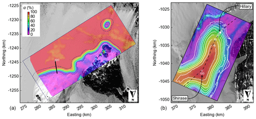
Figure 1 α maps of percentage vertical displacement due to ocean tides. Red colours highlight areas that can be assumed to be freely floating. The white crosses show the tide-model locations that also serve as a common reference point across the images. The solid black line is the location of the profiles shown in Figs. 2 and 3 on the southern McMurdo Ice Shelf (a). The dashed black line shows the location of the profiles along the Darwin Glacier's centerline shown in Fig. 6 (b). The GPS station “Shirase” and “Hillary” in the tidal-flexure zone. White contours delineate areas of constant vertical displacement. The map background is contrast-stretched Landsat 8 panchromatic imagery. The geographic projection is Antarctic Polar Stereographic, with easting and northing coordinates shown in kilometres.

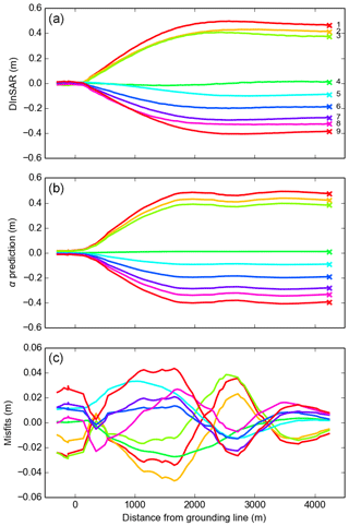
We now extract the α values along the profile from the α map. This α profile can be multiplied with the individual DInSAR measurements on its freely floating end, which results in empirically derived α predictions (Fig. 2b). These mean predictions do not perfectly replicate the DInSAR measurements (Fig. 2a). Their misfits, however, show a very systematic pattern (Fig. 2c). It is desirable to find a combination of offsets that have the least deviation from the α predictions. We therefore hypothesise that this rather systematic signal can be reconstructed using a least-squares strategy. We solve the underdetermined system simultaneously by finding the combination of offsets that result in a minimal sum of squares. The reconstructed offsets must then be removed from the α prediction for the times of SAR data acquisition (Fig. 3a). The computed least-square offsets generally replicate the pattern of the misfits (Fig. 3b) and result in smooth displacement profiles in the ice-shelf grounding zone (Fig. 3c).

Figure 2 Vertical displacements along a profile through the grounding zone of the southern McMurdo Ice Shelf, as (a) measured with nine DInSAR interferograms, (b) predicted from an empirical displacement model (α map) and (c) their difference.

3 Results

In this section we apply the workflow in two spatial dimensions to the Darwin Glacier ($\mathrm{79}{}^{\circ }{\mathrm{53}}^{\prime }$ S, $\mathrm{159}{}^{\circ }{\mathrm{00}}^{\prime }$ E). In this study area, we derived a total of 45 DInSAR images from 12 SAR scenes being acquired on the same satellite track (Table 1). To ensure a balance of both SAR coherence between consecutive images and coverage of different tidal periods in different seasons, we acquired the SAR imagery in two blocks, separated by an 11-week gap. SAR image combinations were generally chosen consecutively so that a later image is always subtracted from an earlier image. For image triples, the central image was taken as a common reference or master image. Additionally the data gap between SAR 8 and 9 was taken into account (no 8–9 combination as loss of coherence over this relatively long interval). The advantage of using every other remaining combination (Table 2) is that more double-differential measurements of tidal amplitude are available for the least-squares fitting algorithm than only using consecutive pairs alone. The system of linear equations is then overdetermined. A dedicated field campaign was conducted in the Darwin Glacier grounding zone in 2016, and in situ data are available for numerical modelling and field validation purposes. In contrast to the simple geometry at the SMIS, the Darwin Glacier consists of a feature-rich embayment that is constrained by steep topography at its margins. Additionally a buttressing ice rise to the Ross Ice Shelf restricts outflow in the North.

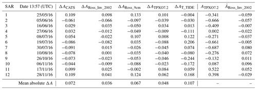
Table 1 SAR imagery used for the Darwin Glacier, least-squares adjustment (ΔA in m) for five tide models, tidal amplitude (A in m) as predicted with the TPXO7.2 tide model and rate of tidal change ($\dot{A}$ in m h⁻¹) as predicted with the Ross_Inv_2002 tide model.

3.1 Reconstruction of displacement maps during satellite overpasses

From the interferogram dataset, we identify a corridor of only about 2 km width along the centerline where the glacier can be assumed to be freely floating (Fig. 1). This area is expected to experience the full oscillation predicted from tide models. We run five tide models to predict the tidal oscillation at the GPS station “Shirase” over the time span of SAR data acquisitions. Here we use atmospheric pressure data from the automatic weather station “Marilyn”, which is located about 120 km away on the Ross Ice Shelf, to correct for the inverse barometric effect. This record correlates well (Pearson's correlation coefficient: 0.989) with a mean of seven barometers installed over 14 d across the Darwin Glacier during the TIDEx campaign. All tide-model predictions show a clear fortnightly occurring spring-neap tidal cycle which is superimposed by a dominant diurnal signal (Fig. 4). The approximately fortnightly spring-neap tidal cycle is primarily determined by the difference in frequency between the dominant K₁ and O₁ diurnal constituents.

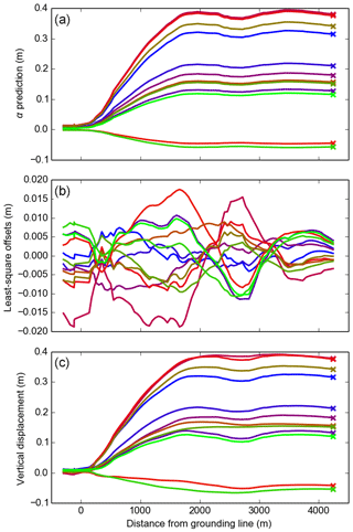
Figure 3 Reconstruction of vertical displacement along the profile during the 12 times of satellite overpasses on the southern McMurdo Ice Shelf. (a) A combination of an empirical displacement model with adjusted CATS2008a tide-model output, (b) their least-square adjustment and (c) the final vertical displacement profiles during the times of SAR data acquisition.

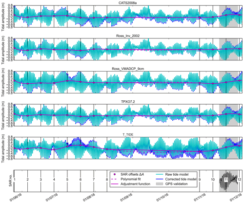
Figure 4 The tidal oscillation at the Darwin Glacier as predicted by four tide models and a harmonic analysis of GPS data from the freely floating area. The tide-model outputs are adjusted to match DInSAR observations using a least-squares fitting technique published by Wild et al. (2018). Black vertical lines coincide with times of SAR data acquisitions. Values for the prevailing tidal amplitudes and their adjustment at these times are given in Table 1. Grey shaded areas delineate the duration of the TIDEx campaign, when GPS data were acquired for validation (Figs. 7 and A1).

We apply T_TIDE to our 16 d record of the Shirase GPS to test the potential of short-term GPS surveys to improve current Antarctic tide models. The problem with using such a short window to determine a full set of tidal constituents results from the interplay of the lunar diurnal tide (Hillary; 23.93 h) with the solar diurnal tide (P₁; 24.07 h), as they are close in frequency and P₁ has an amplitude of 15 %–20 % of K₁. Without accounting for their inference, T_TIDE just extracts an apparent K₁ from a 16 d record that is really K₁+P₁. As a consequence, the K₁ tide from our harmonic analysis can vary by 30 %–40 % over a 6-month period, and its amplitude is only controlled by the exact time that the GPS data were acquired within the K₁+P₁ modulation cycle. Additionally, harmonic decomposition of GPS data is subject to inaccuracies itself, with errors in both the extracted amplitudes and phases. These errors were found to be of the same magnitude as the K₁+P₁ inference. For this reason, we did not use inference to separate K₁ and P₁ (or similarly to separate the semi-diurnal S₂ and K₂ constituents) but perform a thorough analysis on the identified uncertainty range. While the analysis captures the dominant K₁ constituent in the Ross Sea within a reasonable signal-to-noise ratio, fortnightly harmonics could not be retrieved adequately from this time series alone. The T_TIDE prediction is therefore the least accurate tide model and requires the largest adjustment to match DInSAR (Table 1). Although all the corrected tide-model outputs now replicate our DInSAR measurements, their rate of tidal change is affected by the adjustment. Offsets computed for the Ross_Inv_2002 tide model are generally below 10 cm, whereas other tide models require adjustments of up to 13.3 cm (Table 1). This agrees well with the findings of Han et al. (2013), who find that the Ross_Inv_2002 model is the optimum tide model for the Terra Nova Bay, with a 4.1 cm RMSE against 11 d of tide gauge data. We therefore choose Ross_Inv_2002 for numerical modelling purposes to minimise any effects on a viscoelastic model but use TPXO7.2 to reconstruct vertical displacement at the times of satellite overpasses, as it fits best to our GPS measurements. We refer to the Appendix for a validation of individual tide-model outputs with GPS data from Shirase (Fig. A1).

After the adjustment, modelled tidal amplitudes range from −0.966 to 0.781 m over the whole SAR period (Fig. 4). Mean absolute residual error to the 45 DInSAR measurements at the tide-model location Shirase is just 7 mm (Table 2), which can be explained by interferogram noise. We attribute this accuracy to the exceptionally high phase coherence of the TerraSAR-X dataset. The reconstruction algorithm results in 12 smooth vertical displacement maps for the times of SAR data acquisition (Fig. 5).

Table 2 DInSAR images of the Darwin Glacier. The SAR combination from 12 available SAR images, and the tidal amplitude (A in m) as measured at the Shirase location as well as predicted with the TPXO7.2 tide model.

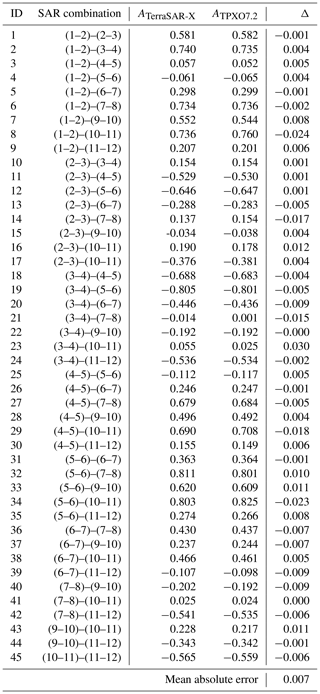
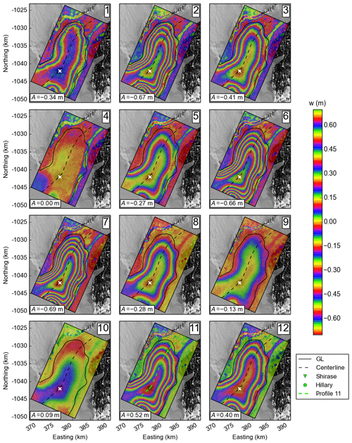
Figure 5 Reconstructed vertical displacement maps in the grounding zone of the Darwin Glacier. The images show surface displacement due to ocean tides at the 12 times of SAR data acquisition. Dashed black lines along the glacier's centerline correspond to the profiles shown in Fig. 6. The white cross marks the tide-model location. The green triangle and dot in the lower centre panel mark the locations of the two GPS stations Shirase (freely floating) and Hillary (within the tidal-flexure zone). Finite-element mesh in grey; mean course of the grounding line as determined from 45 DInSAR images in black. Note the ice rise in the bottom left corner of every panel. The map background is contrast-stretched Landsat 8 panchromatic imagery.

3.2 Validation with GPS measurements

We now validate these reconstructions with available field data. As both GPS records overlap with the acquisition of SAR image 11, we extract the vertical displacement along the glacier's centerline and plot the profiles against the two GPS point measurements. The GPS measurement at Hillary is 0.169 m, which is close to the reconstruction of 0.156 m. The Shirase GPS measurement is 0.566 m, which is slightly above the reconstruction of 0.522 m. We attribute the deviations of +1.3 and +4.4 cm, respectively, to a combination of interpolation artefacts, temporal smoothing of the GPS data and residual errors of the least-squares algorithm. The overall shape of the vertical displacement is well reproduced, as observed with both GPS measurements (Fig. 6).

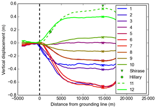
Figure 6 Profiles through the reconstructed maps of vertical displacement along the Darwin Glacier's centerline. The crosses mark the location where the adjusted tide-model output is applied to the α map. The green triangle and dot mark the locations of the two GPS stations Shirase and Hillary and are only used to validate the dashed green profile 11.

3.3 Applications

3.3.1 Tide-model refinement

A map of the tide-deflection ratio (α map) can be combined with the tide model to predict an average time series of vertical displacement between the times of SAR image acquisition. With this approach, the coarse grid of traditional tide models is refined to resolve small-scale features of vertical tidal displacement throughout the embayment. The α value for the pixel containing the Hillary GPS station is 46.06 %. We use this value and linearly scale the adjusted tide-model output for the location of the Shirase GPS to predict vertical tidal motion within the flexure zone. This scaling maintains the tide model's high correlation (Pearson's correlation coefficient: 0.95) with the Shirase record but improves the RMSE between the TPXO7.2 output and the Hillary record from 21.4 to 5.6 cm, which corresponds to an improvement of 74 % to GPS data (Fig. 7). The primary reason for this large improvement, however, is that the tide model now takes the damping of the tidal signal by ice mechanics in the grounding zone into account.

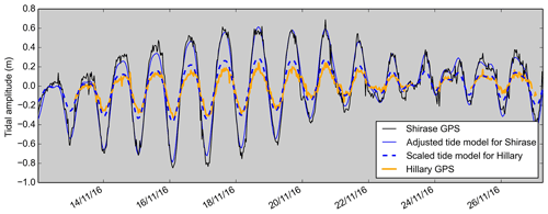
Figure 7 Time series of vertical tidal displacement on the freely floating part of the Darwin Glacier (Shirase) and within the flexure zone close to the grounding line (Hillary) . The (solid blue) corrected tide-model output for the Shirase location is at first compared to (black) its corresponding GPS record. The (dashed blue) extended tide model is scaled and shows an empirical prediction for (orange) the GPS record at the flexure-zone station Hillary. The length of the record corresponds to the grey-shaded area in Fig. 4.

3.3.2 Ice heterogeneity

With the 12 reconstructed displacement maps at hand, it is now possible to perform any image combination. We mosaic the 45 double differences corresponding to DInSAR combinations (Table 2) to allow a more direct comparison between measured and modelled interferograms. SAR image combinations were chosen so that the loss of coherence between SAR 8 and 9 was taken into account and that a maximum number of consecutive, double-differential interferograms were available for the least-squares fitting routine. The synthetic interferograms replicate not only simple tidal fringes as measured with DInSAR but also show complicated viscoelastic signals within the grounding zone (Fig. 8). For an overall assessment of model performance we calculate again the misfit between each modelled and observed interferogram for every pixel, but this time after using the adjusted tide-model output. The standard deviation of these misfits is shown in Fig. 9, with the majority of the glacier surface below the noise level of interferograms (σ<1.0 cm). We identify a narrow band with higher standard deviations (σ≈2.0 cm) from the shear margin of the Darwin Glacier near Diamond Hill, extending along the flow direction onto its ice shelf. Standard deviations are largest in the shear zone of the fast-flowing Ross Ice Shelf and above steep rocky cliffs (σ>4.0 cm), which is a result of poor phase coherence or layovers in SAR images in these areas.

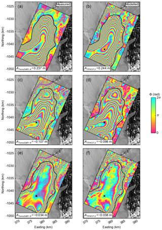
Figure 8 Selection of three measured and modelled images from 45 available DInSAR combinations. Panels (a) and (b) show conditions at a relatively large double-differential tidal amplitude (ID 37), panels (c) and (d) display a pronounced viscoelastic signal in the Darwin Glaciers grounding zone (ID 39), and panels (e) and (f) show a complex flexural pattern (ID 15).

3.3.3 Detection of errors in phase unwrapping

We now extend the earlier one-dimensional analysis of the SMIS to a two-dimensional re-analysis of the SMIS dataset and calculate misfits of nine DInSAR interferograms. Resulting standard deviations are generally smaller in this area (σ<0.3 cm) and smoothly distributed throughout the map. We identify two regions of phase discontinuities between adjacent cells at the SMIS. Both extend from the centre of an ice rise towards Black Island (cyan and green areas in Fig. 9) with σ≈0.4 cm and σ≈0.5 cm. We interpret these rapid spatial gradients as a proxy for errors in the DInSAR measurements, as the modelled least-square interferograms originate from a bivariate spline approximation over a rectangular mesh which acts to minimise curvature. We re-evaluate the remote-sensing part of the analysis and find discontinuities in DInSAR interferograms ID 1 and ID 8 that match the two phase jumps in the standard deviation map. These discontinuities, in turn, occurred during phase unwrapping and can now be corrected.

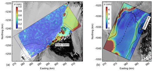
Figure 9 Standard deviations of misfits between modelled and observed DInSAR interferograms. Mean course of the grounding line as determined from DInSAR images in black. (a) Note the ice rise in the upper right corner and two jumps in standard deviations between this ice rise and the dry land for the southern McMurdo Ice Shelf. (b) Note the band of higher standard deviations from the Darwin Glacier's shear margin from Diamond Hill towards the ice rise in the bottom left corner and the high standard deviations. The map background is contrast-stretched Landsat 8 panchromatic imagery.

3.4 Finite-element modelling of viscoelasticity

We hypothesise that any non-linear signal due to viscoelastic ice properties is significantly reduced or even completely lost during the averaging step to compute the α map. This signal can then be reconstructed by finding the offsets to match observations made with DInSAR. We therefore subtract the α prediction again from the 12 reconstructions to extract the theorised viscoelastic signal (Fig. 10). This signal is negligible at times during neap tide (SAR 4 and 9) but well pronounced for SAR images acquired during spring-tide periods (SAR 1, 6, 7, 10 and 11).

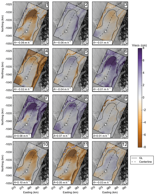
Figure 10 Spatial distribution of 12 least-square offsets that minimise the sum of misfits between 45 maps of α predictions and their corresponding DInSAR measurements. These offsets can be interpreted as the viscoelastic contribution to the reconstructed vertical tidal displacement at the times of SAR data acquisition. Dashed black line corresponds to the glacier's centerline; the solid black line shows the Darwin Glacier's mean grounding line as determined with DInSAR.

In order to further explore this pattern, we now make use of the tiltmeter array and ApRES network of ice-thickness measurements at the Darwin Glacier (Fig. 11). We match the numerical solutions from two finite-element models to seven tiltmeter records, with the goal of deriving information on the physical properties of Antarctic ice. Thereby, Young's modulus, E, is a measure of ice stiffness and controls the width of the flexure region. The value for ice viscosity, ν, influences the timing of the flexural response within the grounding zone (Wild et al., 2017). Two numerical models of ice-shelf flexure are employed. The elastic approximation (Holdsworth, 1969; Vaughan, 1995; Schmeltz et al., 2002) as formulated by Walker et al. (2013) is

$$\begin{array}{}\text{(1)}& k\mathit{w}+{\mathrm{\nabla }}^{\mathrm{2}}\left(\mathit{D}{\mathrm{\nabla }}^{\mathrm{2}}\mathit{w}\right)=\mathit{q},\end{array}$$

where w(t) is the time-dependent vertical deflection of the neutral layer in a plate, ∇² is the Laplace operator in 2-D space and k=5 MPa m⁻¹ a spring constant of the foundation, which is zero for the floating part. The applied tidal force q(t) is defined by

$$\begin{array}{}\text{(2)}& \mathit{q}={\mathit{\rho }}_{\mathrm{sw}}g\left[A\right(t)-\mathit{w}],\end{array}$$

with g=9.81 m s⁻² being the gravitational acceleration and A(t) the time-dependent tidal amplitude given by the adjusted Ross_Inv_2002 tide model. We choose this model, in contrast to the TPXO7.2 model, for finite-element simulations to minimise any potential effects of tide-model adjustment on viscoelasticity (Table 1). The stiffness of the ice shelf is given by (Love, 1906, p. 443)

$$\begin{array}{}\text{(3)}& \mathit{D}={\displaystyle \frac{E{\mathit{H}}^{\mathrm{3}}}{\mathrm{12}(\mathrm{1}-{\mathit{\lambda }}^{\mathrm{2}})}},\end{array}$$

where E is Young's modulus for ice, H(x,y) our ice-thickness map derived from ApRES point measurements and λ=0.4 Poisson's ratio. We compare the elastic model with the viscoelastic approach developed by Walker et al. (2013):

$$\begin{array}{}\text{(4)}& \begin{array}{rl}{\displaystyle \frac{\partial }{\partial t}}& \left[k\mathit{w}+{\mathrm{\nabla }}^{\mathrm{2}}\left(\mathit{D}{\mathrm{\nabla }}^{\mathrm{2}}\mathit{w}\right)\right]+{\displaystyle \frac{Ek}{\mathrm{2}\mathit{\nu }(\mathrm{1}-{\mathit{\lambda }}^{\mathrm{2}})}}\mathit{w}={\displaystyle \frac{\partial }{\partial t}}\mathit{q}\\ & +{\displaystyle \frac{E}{\mathrm{2}\mathit{\nu }(\mathrm{1}-{\mathit{\lambda }}^{\mathrm{2}})}}\mathit{q},\end{array}\end{array}$$

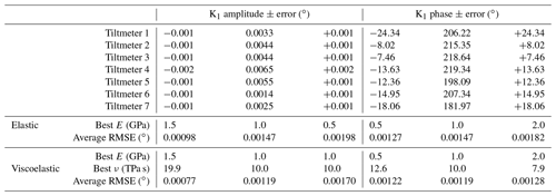
where ν is ice viscosity. The following boundary conditions are applied for both models: the upstream boundary of the model domains on the grounded portion are anchored rigidly ($w=\mathrm{0},{\mathrm{\nabla }}^{\mathrm{2}}w=\mathrm{0}$), and the downstream boundaries on the freely floating ice shelf are set free. The location of the tide-model computation is constrained to be equal to the tidal oscillation ($w=A\left(t\right),\mathrm{\nabla }w=\mathrm{0}$), and the grounding line is represented by a fulcrum (w=0). Both models are implemented in two spatial dimensions to capture the effects of complex grounding-line configuration on ice-shelf flexure (Wild et al., 2018). We then solve the models using the commercial finite-element software COMSOL Multiphysics. As tiltmeters measure slope, w^′, along their longitudinal axis, we derive the models' solutions for vertical displacement, w, with respect to the x and y directions. This allows us to retrieve surface slopes components in the easting and northing direction and to rotate them into the individual orientations of the tiltmeter sensors. With our 16 d tiltmeter records, it is only possible to capture their diurnal components with confidence. Semidiurnal, fortnightly and monthly harmonics have been removed from the tiltmeter time series, and we focus further analysis only on the K₁ component within the 16 d window. Therefore, we now make extensive use of the T_TIDE program to automatically extract the modelled K₁ harmonics from the modelled surface slopes and compare them against the K₁ constituents from the tiltmeters. We thereby take amplitude and phase errors that originate from the harmonic analysis of noisy tiltmeter records into account and find the best rheological parameters to match the elastic and viscoelastic models to these seven K₁ components. Incorporating viscoelastic effects into the model simulations always improves the elastic fit to the tiltmeter data within the uncertainty range of K₁ amplitude and phase (Table ). We find that an average value of Young's modulus of $E=\mathrm{1.0}\pm \mathrm{0.56}$ GPa and an ice viscosity value of $\mathit{\nu }=\mathrm{10}\pm \mathrm{3.65}$ TPa s fit best to our measurements within uncertainty (Fig. ). The viscoelastic model gives an average RMSE of 0.00119^∘ to the seven tiltmeters and improves on the elastic approximation with an average RMSE of 0.00147^∘ by ≈20 %.

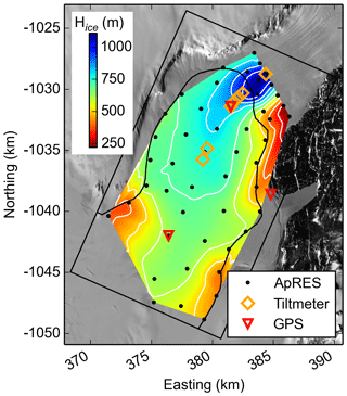
Figure 11 Measured ice-thickness map in the grounding zone of the Darwin Glacier. Black dots show locations of high-precision ApRES measurements. Orange rectangles mark seven tiltmeter sensors that are oriented along the glacier's centerline. Red triangles show locations of GPS stations on the moving ice (Shirase and Hillary) and the location of the GPS base station on stagnant ice which is used for differential correction of the measurements. White contours correspond to a 100 m change in interpolated ice thickness. The map background is contrast-stretched Landsat 8 panchromatic imagery.

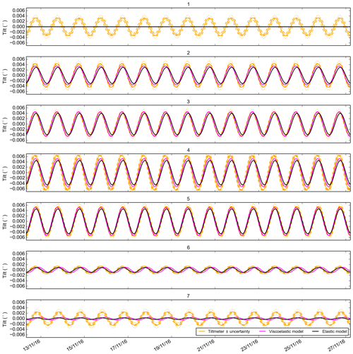
Figure 12 Surface flexure of the K₁ tidal constituent along the Darwin Glacier's centerline as (orange) measured with an array of seven tiltmeters, (magenta) modelled using a viscoelastic rheology and (black) modelled with the elastic approximation. The orange dashed lines correspond to the uncertainty range of the K₁ phases as determined from harmonic analysis of the individual tiltmeter records.

Table 3 Amplitude and phase of the K₁ tidal constituents from harmonic analysis of tiltmeter measurements and values of the rheological parameters to minimise the average RMSE. Amplitudes are given in degrees; phases are the phase lag of the K₁ constituent with respect to the equilibrium tide on Greenwich longitude.

4 Discussion

4.1 Seasonal bias in α map

Due to the alignment of the satellite overpasses with the dominant diurnal tidal constituents in the Ross Sea, the observed stage of the tidal oscillation varies only slowly throughout the year. In the austral winter months, TerraSAR-X images have been acquired during stages of low tide, whereas satellite overpasses concur with stages of high tide during the austral summer months. The first eight snapshots of our SAR data acquisitions for the Darwin Glacier show conditions at low tide, and only the last four are acquired during high tide. For this reason, 21 of our 45 DInSAR images result from low-tide SAR combinations, and only 3 were from purely high-tide SAR combinations. The remaining 21 DInSAR images result from a combination of low- and high-tide SAR snapshots (Table 2). Our α map, as an average of all 45 DInSAR images, ignores this seasonality and may therefore have a low-tide bias. As a result, the contribution of a possible tide-induced landward migration of the grounding line may be affected by the averaging process. The seasonal bias would then modify the scaling of the tide model within the flexure zone. This is supported by the finding that low-tide stages in the Hillary GPS record are matched closely by the scaled tide model, but peaks during high-tide stages are still overestimated (Fig. 4).

4.2 Viscoelasticity between snapshots

Similarly, the linear scaling using an α map only modifies the predicted tidal amplitude but neglects a viscoelastic time delay in the flexural response towards the grounding line. Wild et al. (2017) found that viscosity is most pronounced in the diurnal tidal components. Harmonic analysis of our GPS records reveals that the diurnal K₁ and O₁ constituents at Hillary are lagging approximately 20 min behind Shirase. This signal is currently disregarded in the scaling workflow, as ice is treated as a perfect elastic material that transfers tidal forcing instantaneously in the flexure zone. This assumption, however, allowed us to improve the accuracy of the predicted displacement by 74 %. Currently, the viscoelastic signal can only be reconstructed for the times of SAR data acquisition. Including viscoelasticity between times of satellite overpasses offers a small, but systematic, opportunity for further refinement. In our study area, the rate of tidal change is up to 10 cm h⁻¹ (Table 1), and the viscoelastic misfit corresponding to 20 min time delay is therefore up to about 3 cm.

When separating the viscoelastic contribution from the reconstructed maps of vertical displacement at times of satellite overpasses, we assume that an α prediction corresponds to an instantaneous elastic response. This is justified by viscoelasticity being most pronounced when rates of tidal change are maximal. By expressing the viscoelastic misfits in percentage of prevailing tidal amplitude during the times of satellite overpasses, the areas of pronounced viscoelastic effects can be visualised. They are most pronounced within the Darwin Glacier's shear zone (Fig. 13).

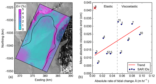
Figure 13 Map of average error due to viscoelasticity in percentage of tidal amplitude (a) and average error on the floating part of the Darwin Glacier versus rate of tidal change as predicted with the adjusted Ross_Inv_2002 tide model (b). Image 6 is considered an outlier and was excluded from the calculation of the linear trend.

When predicting rates of tidal change using the adjusted Ross_Inv_2002 tide model, we identify a threshold of $\dot{A}\approx \pm \mathrm{0.05}$ m h⁻¹ (SAR times 1, 2, 7, 8, 10 and 11 in Table 1) above which viscoelasticity is well represented in the reconstructed vertical displacement maps (panels 1, 6, 7, 8, 10 and 11 in Fig. 10). Image 6 is thereby an exception, as the adjustment of the Ross_Inv_2002 tide model was large (−0.082 m), which affects the viscoelastic model. We find that the error due to viscoelasticity on the floating part of the ice shelf increases with the absolute rate of tidal change (Fig. 13). SAR images acquired during periods of spring tides at the Darwin Glacier show also a significant viscoelastic contribution that diminishes during neap tide periods. These independent observations from satellite data alone support our suggested threshold of ±0.05 m h⁻¹ for the separation of elastic and viscoelastic signals, as derived from tiltmeter data on the southern McMurdo Ice Shelf presented in an earlier study (Fig. 8 in Wild et al., 2017). The advantage of separating the elastic from the viscoelastic contribution to the tidal-flexure pattern is the large potential for improving current inverse modelling techniques to determine grounding-zone ice thickness from DInSAR measurements alone. Hereby, an elastic model is currently employed to optimise grounding-zone ice thickness to match the surface flexure from DInSAR. The applicability of an elastic model varies from location to location, as effective viscosity is dependent on ice temperature and shear stress (Marsh et al., 2014). Our method to separate the two contributions to the flexure pattern may therefore help in removing the viscoelastic contamination and allow purely elastic inverse modelling. Such an analysis, however, goes beyond the scope of this paper and will be published elsewhere.

4.3 Large-scale ice anisotropy

Fast-moving glacial environments like the Darwin Glacier are subject to large deformation by flow convergence and divergence, ice compression and extension, and lateral shearing at the margins accompanied by fracture under tension and rapid thinning by basal melt. With cumulative deformation, a crystallographic fabric evolves that reflects the glacier's flow history (Alley, 1988) and, with it, strain-dependent mechanical anisotropy of ice. The map of average error due to viscoelasticity, in Fig. 13, shows a narrow band of larger errors extending from the Darwin Glacier's shear margin near Diamond Hill out towards the freely floating ice shelf. As preferred crystallographic orientation develops with strain, effective viscosity decreases by about a factor of 10 compared to initially isotropic polycrystalline ice (Hudleston, 2015). Our analysis of tiltmeter data reveals a 5-fold reduced viscosity at the very dynamic Darwin Glacier compared to an earlier study at the almost-stagnant southern McMurdo Ice Shelf (Wild et al., 2017). We hypothesise that this microscopic process explains the macroscopic response observed here and accounts for the measured glacial heterogeneity within the embayment. Large-scale observations of ice anisotropy, in turn, are currently the missing key to improving parametrisations to account for polar ice anisotropy in ice-sheet flow modelling (Gagliardini et al., 2009).

Other processes have been proposed which lead to ice softening in areas with high strain rates. Thermomechanical modelling suggests that shear heating and consequent thermal softening reduce lateral drag in ice-stream margins (Perol and Rice, 2015). Fracture modelling implies that damage reduces ice viscosity along confined crevassed zones, with consequences on the ice-shelf scale (Albrecht and Levermann, 2014). Full-Stokes viscoelastic modelling shows that Glen's non-linear flow law and tidal stresses in the ice-shelf flexure zone are sufficient to explain large-scale temporal variations in ice dynamics (Rosier and Gudmundsson, 2018). These processes, or a combination of them, might certainly be at play, but they do not explain why a band of higher standard deviations can be observed in the shear zone of the Darwin Glacier which is absent in the flexure zone of the SMIS (Fig. 9). We therefore attribute this difference to ice-fabric reorientation in the shear margin.

4.4 Refining tidal constituents using DInSAR

The idea of using SAR interferometry to derive a full set of tidal harmonics was first laid out in a study of tides in the Weddell Sea (Rignot et al., 2000). The authors discussed that DInSAR images cannot be transformed into individual displacement fields because of the nonuniqueness of the inversion. A large number of independent DInSAR images is required to overcome this problem and to resolve the phase of tidal constituents that are close to the repeat pass of the SAR satellite. For example, multiples of the lunar diurnal constituent K₁ (23.93 h) are relatively close to the exact integer repeat pass of TerraSAR-X (11 d), meaning that the observed amplitude of the K₁ constituent only varies once throughout the year. Consequently, SAR images need to be acquired at least over the duration of 1 year to provide some redundancy for the inversion step of DInSAR images to tidal constituents. However, with an exact 12 h period, the stage of the semidiurnal solar tide, S₂, will always be the same at each satellite pass, making TerraSAR-X and similar satellites with repeat passes of integer days blind to the S₂ constituent. For example Minchew et al. (2017) needed a unique spatially and temporally dense SAR acquisition campaign as well as a priori knowledge of the temporal basis functions from GPS data to empirically determine tidal constituents on the Rutford Ice Stream. The four COSMO-SkyMed satellites in orbit, however, produce repeat passes of 1, 3, 4 and 8 d and are blind to the S₂ constituent as well, even when using >1000 available DInSAR images. Although other dominant tidal constituents like M₂ (12.4 h) and O₁ (25.82 h) were inferred successfully, the method presented here can achieve a higher accuracy of the total tide with fewer DInSAR images.

5 Conclusions and outlook

Accurate prediction of ocean tides in coastal areas around Antarctica is crucial, as the majority of Antarctica's ice is discharged through large outlet glaciers. We presented a data fusion method between DInSAR and traditional Antarctic tide models to predict spatial variability in tidal motion near the grounding line. The primary value of using DInSAR in conjunction with tide models lies in the spatio-temporal benefits of resolving complex grounding-zone deformation. Their symbiosis not only improves current accuracies of the predicted tidal amplitudes in coastal regions generally but also eases issues related to the timing of the tidal wave and the Sun-synchronous satellite orbit when attempting to derive tide-models from SAR data alone. In our study area, the method presented in this paper improves traditional tide modelling on average by 22 % from 11.8 to 9.3 cm RMSE against 16 d of GPS data. The GPS station Shirase on the freely floating part of the Darwin Glacier has proven invaluable in determining which tide model has to be used to best reconstruct the vertical displacement during satellite overpasses. For the Darwin Glacier, the TPXO7.2 tide model predicts the tidal oscillation best. With using DInSAR measurements to adjust the TPXO7.2 tidal prediction, its RMSE could be improved by 39 % from 10.8 to 6.7 cm. Our GPS record from Shirase is too short to improve already-available Antarctic tide models. A longer record is required to adequately resolve a full set of tidal constituents. We produced an empirical displacement map from DInSAR for tidal deflection (α map). Comparison of a GPS record within the tidal-flexure zone (Hillary) with predicted vertical displacement from feeding the α map with the adjusted TPXO7.2 tide model shows a 74 % improvement over using the tide-model output alone. This independent validation supports the finding that our method for making use of DInSAR is very useful for refining tide models in Antarctic grounding zones.

Numerical modelling of ice dynamics in Antarctic grounding zones commonly assumes that ice is isotropic and homogeneous, i.e. of the same density and rheological properties throughout. Our analysis reveals that this assumption is valid for the southern McMurdo Ice Shelf, an almost-stagnant area with a simple grounding-line configuration, but invalid for the Darwin Glacier, a fast-flowing outlet glacier with complex shear margins causing non-negligible ice heterogeneity within the embayment.

Further work is required in order to improve tide models in a larger variety of grounding zones by including effects of grounding-line migration and variability in horizontal ice flow.

Appendix A: GPS evaluation of tide models

The quality of the used tide model to correctly reconstruct tidal displacement at the times of SAR data acquisitions is also crucial to accurately predict spatial variability in tidal motion for all times. Here, we assume that a freely floating area on the ice shelf experiences the full oscillation as predicted from a tide model. In this area, however, tide-model output deviates from our DInSAR measurements. This indicates either that the area under investigation is prevented from a freely floating state by lateral stresses within the embayment or that the tide-model prediction is inaccurate for this area. We circumvent this ambiguity by making use of the high vertical accuracy of DInSAR and correct the tide-model prediction to match our satellite measurements. This raises the question of whether the adjustment improves or worsens the match to a real tidal motion. We therefore independently evaluate the pre- and post-adjustment tide-model predictions and calculate their RMSE to 16 d of GPS data from the freely floating area (Table A1). The adjustment improves all traditional tide-model predictions by up to −39 % for TPXO7.2 and only worsens the RMSE for the T_TIDE output by +11 %, indicating that a harmonic analysis of GPS data cannot be improved by using DInSAR for correction purposes. We choose TPXO7.2 for further processing, as it displays the overall smallest RMSE (6.7 cm) and replicates the small-scale variability observed during the neap tide period in the second half of our GPS record.

Table A1 Root-mean-square errors in metres between tide-model output and GPS data from Shirase before and after the adjustment to match DInSAR.

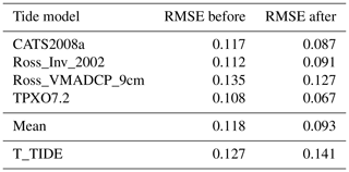
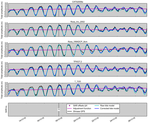
Figure A1 Validation of the tidal predictions of five tide models with a GPS record from the freely floating Shirase station. The tide-model outputs are adjusted to match DInSAR observations using a least-squares fitting technique published by Wild et al. (2018). Root-mean-square errors before and after this adjustment are presented in Table A1. The length of the records corresponds to the grey-shaded area in Fig. 4.