Glacier thickness estimations of alpine glaciers using data and modeling constraints

Advanced knowledge of the ice thickness distribution within glaciers is of fundamental importance for several purposes, such as water resource management and the study of the impact of climate change. Ice thicknesses can be modeled using ice surface features, but the resulting models can be prone to considerable uncertainties. Alternatively, it is possible to measure ice thicknesses, for example, with ground-penetrating radar (GPR). Such measurements are typically restricted to a few profiles, with which it is not possible to obtain spatially unaliased subsurface images. We developed the Glacier Thickness Estimation algorithm (GlaTE), which optimally combines modeling results and measured ice thicknesses in an inversion procedure to obtain overall thickness distributions. GlaTE offers the flexibility of being able to add any existing modeling algorithm, and any further constraints can be added in a straightforward manner. Furthermore, it accounts for the uncertainties associated with the individual constraints. Properties and benefits of GlaTE are demonstrated with three case studies performed on different types of alpine glaciers. In all three cases, subsurface models could be found that are consistent with glaciological modeling and GPR data constraints. Since acquiring GPR data on glaciers can be an expensive endeavor, we additionally employed elements of sequential optimized experimental design (SOED) for determining cost-optimized GPR survey layouts. The calculated cost–benefit curves indicate that a relatively large amount of data can be acquired before redundant information is collected with any additional profiles, and it becomes increasingly expensive to obtain further information.

1 Introduction

Estimating the amount of the glacier ice around the globe is crucial, for example, for sea-level predictions, securing fresh water resources, designing hydropower facilities in high-alpine environments and predicting the occurrence of glacier-related natural hazards. For estimating the overall glacier ice mass and its local distribution, (i) knowledge of the glacier outline, (ii) its surface topography and (iii) the underlying bedrock topography is required. The first two quantities can be observed with aerial and satellite imagery, but the bedrock topography is more difficult to determine.

The conceptually simplest option includes drilling boreholes through the glacier ice (e.g., Iken, 1988). This approach offers ground-truth information, but only a very sparse observation grid can be obtained with realistic efforts. Therefore, geophysical methods have been employed for obtaining more detailed information. Due to the very high electrical resistivity of glacier ice and the relatively high electromagnetic impedance contrast between ice and bedrock material, ground-penetrating radar (GPR) techniques, also referred to as radio-echo sounding, have been the primary choice for such investigations (e.g., Evans, 1963). GPR data can either be acquired using ground-based methods (e.g., Watts and England, 1976), or, more efficiently, using fixed-wing airplanes (e.g., Steinhage et al., 1999) or helicopters (e.g., Rutishauser et al., 2016).

Despite the powerful capabilities of modern GPR acquisition systems, it is still beyond any practical limits to acquire spatially unaliased 3-D data sets. GPR data are therefore collected only along a sparse network of profiles, which leaves considerable uncertainties in the regions between the profiles.

To address this problem, glaciological modeling techniques have been established to relate observable surface parameters to the thickness distribution of ice. One of the earliest concepts was published by Nye (1952). He established a simple relationship between the surface slope and ice thickness. During the past decades, more sophisticated ice thickness modeling techniques have emerged rapidly. Various glaciological constraints, such as mass conservation and/or the relation between basal shear stress and ice thickness, were considered (e.g., Farinotti et al., 2009; Huss and Farinotti, 2012; Clarke et al., 2013; Linsbauer et al., 2012; Morlighem et al., 2011). See Farinotti et al. (2017) for a more complete review of most of the approaches published to date.

Due to inaccuracies of the observed data (GPR measurements, surface topography, etc.) and/or inadequacies in the modeling approaches, modeled ice thicknesses cannot be expected to be perfect. This can be considered by formulating ice thickness estimation as an optimization problem, in which the discrepancies between observed and predicted data are minimized (e.g., Morlighem et al., 2014). In this contribution, we follow an approach similar to Morlighem et al. (2014) but with a different implementation. We introduce the general framework of Glacier Thickness Estimation (GlaTE), with which modeling and data constraints can be combined in an appropriate fashion. After introducing the underlying theory, we demonstrate the performance of the GlaTE inversion procedure with three case studies. In the second part of the paper, we employ elements of GlaTE to address the experimental design problem. Here, we seek a data set to be measured that offers maximum information content at minimal costs. For that purpose, we consider sequentially optimized experimental design (SOED) techniques (e.g., Maurer et al., 2017). The paper concludes with a critical review of potential problems and shortcomings of GlaTE and the associated SOED procedures, and we outline options to address these issues and propose useful extensions of the methodology.

2 GlaTE inversion algorithm

2.1 Theory

The basic idea of GlaTE inversions is to combine observable data with glaciological modeling constraints. A key feature of the algorithm includes appropriate consideration of the uncertainties associated with both constraints. All constraints are formulated, such that they can be integrated into a single system of equations, which can be solved with an appropriate solver.

The first type of constraints includes the GPR data. They can be written in the form of

$$\begin{array}{}\text{(1)}& \mathbf{G}{\mathit{h}}^{est}={\mathit{h}}^{\mathrm{GPR}},\end{array}$$

where h^est is a vector including the unknown (estimated) ice thicknesses at M locations (typically defined on a regular grid R on a glacier) and G is a N^GPR×M matrix with ones in its main diagonal and zeros everywhere else (N^GPR= number of available GPR data points; M= number of elements in h^est). The vector h^GPR of length N^GPR includes the GPR-based thickness estimates. Since the GPR data usually do not coincide with the grid points of R, the values h^GPR are obtained by interpolating or extrapolating the GPR data to the nearest grid points of R.

Next, we consider glaciological modeling constraints. In principle, any of the algorithms proposed in the literature can be employed. Here, we closely follow the approach described in Clarke et al. (2013). Input data include a digital terrain model (DTM, defined on R) and the glacier outline.

First, the glacier area is subdivided into so-called flow sheds using the MATLAB TOPO-Toolbox (Schwanghart and Kuhn, 2010). The subsequent procedure is applied to each flow shed individually (see comments in Clarke et al., 2013, for more information on the flow shed subdivision).

Next, the apparent mass-balance is applied, defined as follows:

$$\begin{array}{}\text{(2)}& \stackrel{\mathrm{̃}}{\mathit{b}}=\dot{\mathit{b}}-{\displaystyle \frac{\partial \mathit{h}}{\partial t}},\end{array}$$

with $\dot{\mathit{b}}$ being the mass balance rate and $\partial \mathit{h}/\partial t$ the thickness change rate, which is either determined by measuring $\dot{\mathit{b}}$ and $\partial \mathit{h}/\partial t$ or computed via the condition

$$\begin{array}{}\text{(3)}& \underset{{\mathrm{\Omega }}_{\mathrm{G}}}{\int }\stackrel{\mathrm{̃}}{\mathit{b}}=\mathrm{0},\end{array}$$

where Ω_G denotes the glacier area (see Farinotti et al., 2009 for more details). In the next step, the flow sheds are partitioned into a prescribed number of elevation zones D_i (i=1… number of elevation zones), for which the ice discharge Q_i through its lower boundary is computed using

$$\begin{array}{}\text{(4)}& Q_{\mathrm{i}}=\underset{{\mathrm{\Omega }}_{D_i}}{\int }\stackrel{\mathrm{̃}}{\mathit{b}},\end{array}$$

where ${\mathrm{\Omega }}_{D_i}$ is the area of zone D_i. Following Clarke et al. (2013), the basal shear stress τ can then be obtained via the relationship

$$\begin{array}{}\text{(5)}& \mathit{\tau }={\left[{\displaystyle \frac{\left(n+\mathrm{2}\right)\mathit{\rho }g\sin {\left(\mathit{\varphi }\right)}^{\mathrm{2}}\mathit{\xi }q}{\mathrm{2}A}}\right]}^{\mathrm{1}/\left(n+\mathrm{2}\right)}.\end{array}$$

The parameters n, ρ, g, and A denote the exponent of Glen's flow law, ice density, gravity acceleration, and creep rate factor, respectively (e.g., Cuffey and Patterson, 2010). The factor ξ denotes the creeping contribution (relative to basal sliding) to the ice flux $\left(\mathrm{0}<\mathit{\xi }<\mathrm{1}\right)$, and q is the specific ice discharge $q_{\mathrm{i}}={\stackrel{\mathrm{‾}}{Q}}_{\mathrm{i}}/l_i$, where l_i is the length of the lower boundary of D_i and ${\stackrel{\mathrm{‾}}{Q}}_{\mathrm{i}}$ is the average of Q_i within D_i. Likewise, the angle ϕ represents the surface slope averaged along the lower boundary of D_i.

As outlined in Kamb and Echelmeyer (1986), the physics of ice flow can be incorporated into the modeling procedure by applying “longitudinal averaging” of the shear stress (i.e., along the flow direction). We apply this procedure to the results obtained with Eq. (5). Finally, the ice thicknesses ${\widehat{\mathit{h}}}^{\mathrm{glac}}$ (glac stands for glaciological modeling constraints) are obtained using

$$\begin{array}{}\text{(6)}& {\widehat{\mathit{h}}}^{\mathrm{glac}}={\displaystyle \frac{{\mathit{\tau }}^{\ast }}{\mathit{\rho }g\sin \left(\mathit{\varphi }\right)}},\end{array}$$

where τ^∗ denotes the basal shear stress after longitudinal averaging.

Some of the parameters in Eq. (5) may be subject to considerable uncertainties. For example, the parameter ξ is often poorly known, and it is not guaranteed that the values of the parameters A and n, usually taken from the literature, are accurate. Typically, n is reasonably well constrained but A can vary over orders of magnitudes. Therefore, the overall magnitudes of ${\widehat{\mathit{h}}}^{\mathrm{glac}}$ may be significantly overestimated or underestimated. This can be considered with an additional factor α_GPR, yielding

$$\begin{array}{}\text{(7)}& {\mathit{h}}^{\mathrm{glac}}={\mathit{\alpha }}_{\mathrm{GPR}}{\widehat{\mathit{h}}}^{\mathrm{glac}}.\end{array}$$

α_GPR can be computed with an optimization procedure that minimizes ${∥{\mathit{h}}^{\mathrm{GPR}}-{\mathit{\alpha }}_{\mathrm{GPR}}{\widehat{\mathit{h}}}^{\mathrm{glac}}∥}^{\mathrm{2}}$.

The correction factor α_GPR accounts for some inadequacies of Eq. (5), but it is still possible that there are systematic differences between h^GPR and h^glac. To avoid the resulting inconsistencies, we consider not the absolute value of h^glac but instead the spatial gradient of ∇h^glac as glaciological constraints, resulting in

$$\begin{array}{}\text{(8)}& \mathbf{L}{\mathit{h}}^{\mathrm{est}}=\mathrm{\nabla }{\mathit{h}}^{\mathrm{glac}},\end{array}$$

where L is a difference operator of dimension M×M .

Further constraints can be imposed via the glacier boundaries that can be determined from aerial or satellite images or ground observations. They are considered in the form of the following equation:

$$\begin{array}{}\text{(9)}& \mathbf{B}{\mathit{h}}^{\mathrm{est}}=\mathrm{0},\end{array}$$

where B is a M×M matrix with ones at appropriate places in its main diagonal.

Depending on the discretization of the glacier models (i.e., the discretization of R), the constraints described above may allow the resulting system of equations to be solved unambiguously. However, in most cases, there will still be a significant underdetermined component, that is, there will be many solutions that explain the data equally well. This requires regularization constraints to be applied (e.g., Menke, 2012). A common strategy for regularizing such problems is to follow Occam's razor, which identifies the “simplest” solution out of the many possible solutions (Constable et al., 1987). Here, we define “simplicity” in terms of structural complexity, that is, we seek a smooth model. This can be achieved via a set of smoothing equations of the form

$$\begin{array}{}\text{(10)}& \mathbf{S}{\mathit{h}}^{\mathrm{est}}=\mathrm{0},\end{array}$$

where S is a M×M smoothing matrix.

All the constraints can now be merged into a single system of equations:

$$\begin{array}{}\text{(11)}& \left(\begin{array}{c}{\mathit{\lambda }}_{\mathrm{1}}\mathbf{G}\\ {\mathit{\lambda }}_{\mathrm{2}}\mathbf{L}\\ {\mathit{\lambda }}_{\mathrm{3}}\mathbf{B}\\ {\mathit{\lambda }}_{\mathrm{4}}\mathbf{S}\end{array}\right){\mathit{h}}^{\mathrm{est}}=\left(\begin{array}{c}{\mathit{\lambda }}_{\mathrm{1}}{\mathit{h}}^{\mathrm{GPR}}\\ {\mathit{\lambda }}_{\mathrm{2}}\mathrm{\nabla }{\mathit{h}}^{\mathrm{glac}}\\ \mathrm{0}\\ \mathrm{0}\end{array}\right),\end{array}$$

where the parameters λ₁ to λ₄ allow a weighting according to the confidence into the individual contributions. The dimension of the system of equations in Eq. (11) can be very large, but the matrices G, L, B and S are all extremely sparse. Therefore, sparse matrix solvers, such as LSQR (Paige and Saunders, 1982) can solve such systems efficiently for h^est. The test data sets, described later, yield matrices including up to $\sim \mathrm{320}\mathrm{000}\times \mathrm{90}\mathrm{000}$ elements. The LSQR algorithm for solving such a matrix required approx. 2 s on a standard PC.

A critical part of the GlaTE inversions includes a proper choice of the weighting parameters λ₁ to λ₄. Parameter λ₃ is not critical and can be fixed to an appropriate value (e.g., 1.0). The magnitudes of the remaining three parameters must be chosen, such that the system of equations in Eq. (11) is solvable. However, it also needs to be considered that the constraints related to λ₁ and λ₂ are subject to significant inaccuracies. It is difficult to predict the accuracy of the modeling constraints, but the accuracy of the GPR data constraints, subsequently denoted as ε^GPR, can usually be quantified. Therefore, we have chosen the following strategy.

1. Initially, we set λ₁=1 and choose a low λ₂ value (i.e., a high λ₁∕λ₂ ratio). Such a ratio indicates a much higher confidence in the GPR data constraints compared with the glaciological modeling constraints. Furthermore, we choose a large value of λ₄, which is expected to oversmooth the ice thickness estimates.

2. With this choice of parameters, a first GlaTE inversion is carried out, and it is checked if a prescribed percentage (e.g., 95 %) of the estimated thicknesses h^est matches the GPR data h^GPRwithin their accuracy limits ±ε^GPR.

3. For an overly high value of λ₄, it cannot be expected that the prescribed percentage of matching data can be achieved. Therefore, λ₄ is gradually lowered until the condition, specified in point 2, is met or a prescribed lower threshold of ${\mathit{\lambda }}_{\mathrm{4}}={\mathit{\lambda }}_{\mathrm{4}}^{min}$ is reached. The final smoothing weight, obtained with this procedure, is denoted as ${\stackrel{\mathrm{‾}}{\mathit{\lambda }}}_{\mathrm{4}}$. Since the λ₁∕λ₂ ratio is still large, it is expected that ${\stackrel{\mathrm{‾}}{\mathit{\lambda }}}_{\mathrm{4}}$ is also large because the modeling constraints do not contribute much to the GlaTE inversion. Essentially, a smooth interpolation of the GPR data between the profile lines is performed.

4. The λ₁∕λ₂ ratio is gradually lowered and step 3 is carried out again (λ₄ is reset to a high initial value). This iterative procedure is repeated until (i) ${\stackrel{\mathrm{‾}}{\mathit{\lambda }}}_{\mathrm{4}}={\mathit{\lambda }}_{\mathrm{4}}^{min}$ without reaching the prescribed data match, or (ii) the λ₁∕λ₂ ratio has reached a prescribed lower limit.

   With decreasing λ₁∕λ₂ ratios, the importance of the glaciological modeling constraints increases, and the contributions of the smoothing constraints need to be lowered to achieve the prescribed data match. Below a certain λ₁∕λ₂ ratio, it will likely no longer be possible to fit a sufficiently large percentage of the data within the limits ±ε^GPR, even when ${\stackrel{\mathrm{‾}}{\mathit{\lambda }}}_{\mathrm{4}}={\mathit{\lambda }}_{\mathrm{4}}^{min}$. If this is not the case, the λ₁∕λ₂ ratio could be lowered to an arbitrary low level, but if the confidence in the glaciological modeling constraints is rather limited, it is possible to define a lower threshold where the GlaTE inversion would stop, even when ${\stackrel{\mathrm{‾}}{\mathit{\lambda }}}_{\mathrm{4}}>{\mathit{\lambda }}_{\mathrm{4}}^{min}$.

With such a strategy, it is possible to achieve several desirable features of glacier thickness estimations, namely

• the GPR data are fitted only within the prescribed accuracy limits and no overfitting is performed,

• the contribution of the glaciological constraints are maximized, and

• the influence of the (unphysical) smoothing constraints is minimized.

2.2 Performance tests

For testing the GlaTE inversion algorithm, we investigated glacier ice thickness at three sites in the Swiss Alps (Fig. 1 and Table 1). The first site is Vadret da Morteratsch (Fig. 1a). Lying at altitudes between 2050 and 4000 m a.s.l. (Zekollari et al., 2013), the glacier has a typical valley-glacier shape and is located in the Engadin region of Switzerland. In 2015, the tributary glacier Vadret Pers, on the eastern part of the main glacier, detached from the main trunk of Vadret da Morteratsch, but we continue to treat both glaciers as a connected system, since the last available outline of the glaciers in 2015 shows the remnant of the former connection. In 2010, the glacier system covered an area of ≈15 km² and had a length of ≈7.4 km.

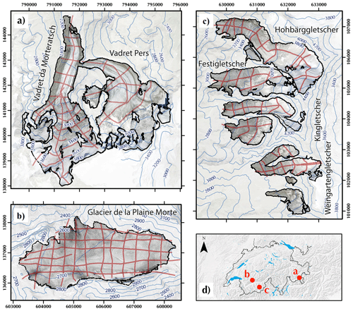
Figure 1 Orthoimages and surface topography isolines of the glaciers investigated: (a) Vadret da Morteratsch, (b) Glacier de la Plaine Morte and (c) the Dom region. The map of Switzerland in panel (d) indicates the locations of the glaciers. GPR profiles acquires are shown in red. Orthophotos © 2017 swisstopo (JD100042). Coordinate system: CH1903.

Table 1 Characteristics and data sets of glaciers investigated. Slope ϕ denotes the average slope angle.

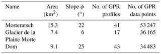
The second site, Glacier de la Plaine Morte (2400–3000 m a.s.l., Fig. 1b), is the largest plateau glacier in the European Alps (Huss et al., 2013). The surface slope is shallow with an average slope angle of about 6^∘ and a short glacier tongue draining towards the north.

The third site is a cluster of small valley flanks and cirque-type glaciers on the eastern flank of the Matter Valley (Fig. 1c) below the Dom peak. From north to south, the glaciers are named Hohbärggletscher, Festigletscher, Kingletscher and Weingartengletscher. The Hohbärggletscher is the largest (2800–4500 m a.s.l.) and longest of the group. The individual glaciers were treated as individual flow sheds during the data analysis, but the α_GPR factor was determined for the entire Dom area.

For all sites, the recorded GPR profiles are shown in Fig. 1. Most of the data were recorded with the dual polarization system AIR-ETH (Langhammer et al., 2018). A grid of profiles was acquired in 2016 on the Glacier de la Plaine Morte and in 2017 on the Vadret da Morteratsch and in the Dom Region. The data were processed as described in Grab et al. (2018), and the bedrock depths and the corresponding ice thicknesses were obtained from the migrated GPR images.

As input data for the glacier models, surface topography and an outline of the individual glaciers was required. As surface topography, we used the swissALTID3D (DTM, Digital Terrain Model Release 2017 © swisstopo, JD100042). The most recent version, covering the individual glaciers, was extracted and down-sampled to 10 m resolution. The outline represents the extension of the glacier in 2015–2016. DTM and glacier outlines are displayed in Fig. 1. In accordance with Farinotti et al. (2009), we employed mass balance gradients of 0.05 and 0.09 in the accumulation and ablation zones, respectively.

As an appropriate measure of the accuracy of the GPR data, we considered a relative (depth-dependent) quantity ${\mathit{\epsilon }}^{\mathrm{GPR}}=∥{\mathit{h}}^{\mathrm{glac}}-{\mathit{h}}^{\mathrm{GPR}}∥/\left({\mathit{h}}^{\mathrm{GPR}}+h^{min}\right)$, where h^min is a minimum thickness to avoid unreasonably large relative errors at shallow depths. Values of ε^GPR=0.05 and $h^{min}=\mathrm{5.0}$ were judged to be adequate. For all three data sets, we employed ${\mathit{\lambda }}_{\mathrm{4}}^{min}=\mathrm{4.0}$ and the prescribed data fit was 95 %. This could be achieved with a minimum λ₁∕λ₂ ratio of 3.0 (initial values for λ₄ and λ₁∕λ₂ were 50.0 and 5.0).

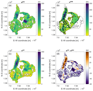
Figure 2 Results from Vadret da Morteratsch using only (a) glaciological constraints or (b) GPR constraints. Panel (c) shows the GlaTE inversion result, and panel (d) depicts the difference between the results shown in panels (a) and (c). Colors indicate ice thickness or ice thickness differences. Available thickness data obtained from GPR profiles are marked with black lines in panel (b).

Figure 2 shows the ice thicknesses distributions, when only glaciological constraints are applied (h^glac, Fig. 2a), when only GPR constraints are considered (h^GPR, Fig. 2b), results from the GlaTE algorithm (h^est, Fig. 2c) and considering the difference between h^glac and h^est (Fig. 2d). In Fig. 2b, the thicknesses were obtained by natural neighbor interpolation from the GPR data. Since no extrapolation was performed, not all glacierized regions have an ice thickness estimate. h^glac and h^GPR exhibit increased thicknesses in the western glacier, but only the glaciological constraints indicate an overdeepening in the eastern glacier, thereby indicating that the two models are inconsistent. The results from the GlaTE inversion (h^est, Fig. 2c) demonstrate that it is possible to find a smooth model that satisfies both the glaciological and the GPR data constraints.

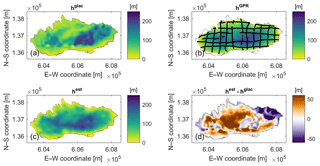
Figure 3 Results from Glacier de la Plaine Morte using only (a) glaciological constraints or (b) GPR constraints. Panel (c) shows the GlaTE inversion result, and panel (d) depicts the difference between the results shown in panels (a) and (c). Colors indicate ice thickness or ice thickness differences. Available thickness data obtained from GPR profiles are marked with black lines in panel (b).

The corresponding results for the Glacier de la Plaine Morte are shown in Fig. 3. The glaciological model suggests a deep isolated trough slightly east of the center (Fig. 3a). This is not supported by the GPR data, which instead indicate a larger E–W-oriented elongated zone of increased thickness (Fig. 3b). Such a feature is also contained in the GlaTE inversion results (Fig. 3c). Furthermore, the glaciological model in Fig. 3a overestimates the ice thickness in the northeastern part of the glacier.

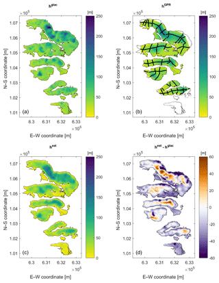
Figure 4 Results from Dom region using only (a) glaciological constraints or (b) GPR constraints. Panel (c) shows the GlaTE inversion result, and panel (d) depicts the difference between the results shown in panels (a) and (c). Colors indicate ice thickness or ice thickness differences. Available thickness data obtained from GPR profiles are marked with black lines in panel (b).

Results from the Dom region show a relatively good match between the glaciological model (Fig. 4a) and the GlaTE inversion result (Fig. 4c). The glaciological model tends to underestimate the maximum thickness in the center of the glacier tongues and overestimate the thickness towards the edges (Fig. 4d). The isolated trough structures (ice thickness >200 m) in the northernmost glacier in the glaciological model (Fig. 4a) are only partially supported by the GPR data (Fig. 4b) and the GlaTE inversion (Fig. 4c). In the southernmost Weingartengletscher, no data constraints exist (Fig. 4b). The nonzero differences in this part (Fig. 4d) are the result of the smoothing constraints. Here, the thickness estimates from the glaciological model are thus more trustworthy.

3 Optimized experimental design using GlaTE inversion

All the investigations, described in Sect. 2, were based on existing GPR data. Their experimental layouts were designed heuristically using experience from prior surveys. Once a glacier model has been established, one may realize that another GPR survey layout may have provided better information. Therefore, a dense survey grid, as employed for 3-D seismic reflection campaigns for hydrocarbon exploration (e.g., Vermeer, 2003) would be the best choice. This, however, would exceed by far the budgets typically available for glacier investigations.

Optimizing the glaciological constraints with only a limited number of GPR data is a chicken-and-egg problem: identifying the most useful GPR data to be added would require knowledge on where the true ice thickness distribution deviates most from the distribution in the glaciological model, but this would require advanced prior knowledge about the ice thickness that one wants to measure. The problem can be tackled nevertheless by making some specific assumptions (see below).

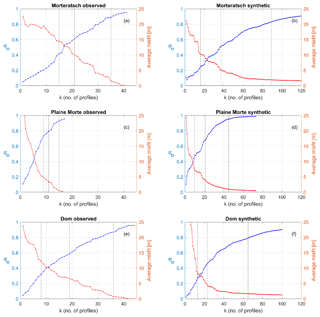
Figure 5 Evolution of data fit d^fit (blue curves) and average data misfit $\mathrm{mean}\left({\mathit{h}}^{{\mathrm{est}}_k}-{\mathit{h}}^{\mathrm{true}}\right)$ (red curves). Panels (a), (c) and (e) show the results for the observed data, and panels (b), (d) and (f) show the results for the synthetic data generated on a densely spaced grid of hypothetical profiles. Vertical dashed lines indicate the number of profiles required to achieve d^fit values of 0.5, 0.7 and 0.9 (see also Figs. 6 to 11).

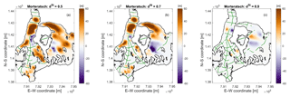
Figure 6 Vadret da Morteratsch model misfit ${\mathit{h}}^{\mathrm{true}}-{\mathit{h}}^{{\mathrm{est}}_k}$ after selected stages of the experimental design procedure using observed data (see also vertical dashed lines in Fig. 5). The selected GPR profiles are superimposed with green lines.

With our investigations, we address the following questions.

1. Was the experimental geometry and the amount of data acquired in the three investigation areas adequate?

2. Do better experimental layouts exist for constraining the ice thicknesses in a cost-optimized manner?

3. Can some general recommendations be made for designing helicopter-borne GPR surveys on glaciers?

Due to the lack of knowledge on the true ice thicknesses, we assumed that the GlaTE inversion results, shown in Figs. 2, 3 and 4 are a good proxy for the actual thickness distributions. Without GPR data, the state of knowledge is represented by the glaciological model (Figs. 2a, 3a and 4a). For these models, only 12 % (Morteratsch), 8 % (Glacier de la Plaine Morte) and 14 % (Dom) of the GPR data constraints satisfy the condition $∥{\mathit{h}}^{\mathrm{glac}}-{\mathit{h}}^{\mathrm{GPR}}∥/\left({\mathit{h}}^{\mathrm{GPR}}+h^{min}\right)<{\mathit{\epsilon }}^{\mathrm{GPR}}$, and the average ice thickness misfits over the entire glacier area (mean(h^glac−h^true)) (h^true= “true” model) are 22, 32 and 23 m for the three data sets, respectively. It should be noted that the glaciological models h^glac have been calibrated with α_GPR. If no GPR data were to be available, the performance of the glaciological models would have been even worse.

Subsequently, we analyzed which of the profiles j (j=1… nprof, number of profiles) causes the largest discrepancies between h^GPR and h^glac. For that purpose we define

$$\begin{array}{}\text{(12)}& d_{\mathrm{1}}^{\mathrm{cost}}=\underset{j}{max}\left({\displaystyle \frac{\sum _{i=\mathrm{1}}^{i=n_j}P\left(\left|h_{ij}^{\mathrm{GPR}}-h_{ij}^{\mathrm{glac}}\right|/h_{ij}^{\mathrm{GPR}}\right)}{c_j}}\right),\end{array}$$

where index i runs over all n_j data points of profile j. $h_{ij}^{\mathrm{GPR}}$ and $h_{ij}^{\mathrm{glac}}$ represent the measured and modeled ice thickness at data point i of profile j, respectively. The function P is defined as

$$\begin{array}{}\text{(13)}& P\left(x\right):=\left\{\begin{array}{ll}\mathrm{1}& \text{if }x>{\mathit{\epsilon }}^{\mathrm{GPR}}\\ \mathrm{0}& \text{if }x\le {\mathit{\epsilon }}^{\mathrm{GPR}}\end{array}\right.\end{array}$$

Since longer profiles would be associated with higher (monetary) data acquisition costs, the discrepancy $d_{\mathrm{1}}^{\mathrm{cost}}$ is normalized with a cost factor c_j, defined as

$$\begin{array}{}\text{(14)}& c_j=max\left({\mathrm{len}}_j,\mathrm{200}\right),\end{array}$$

where len_j represents the length of profile j. This cost function assumes that the acquisition costs increase linearly with profile length, which is realistic because the helicopter costs are typically charged per minute of flight time. To avoid overly short profiles dominating $d_{\mathrm{1}}^{\mathrm{cost}}$, the assumption was made that profiles with a length <200 m would incur the same costs (for such short profiles the flight time is typically governed by positioning the helicopter at the starting point of a profile).

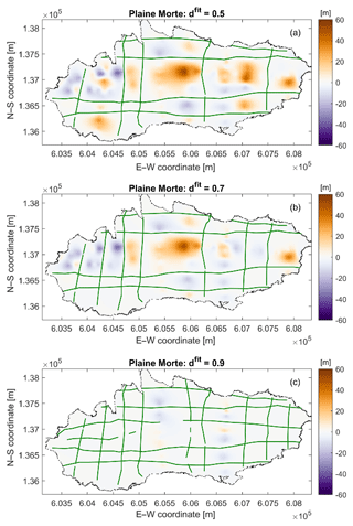
Figure 7 Glacier de la Plaine Morte model misfit ${\mathit{h}}^{\mathrm{true}}-{\mathit{h}}^{{\mathrm{est}}_k}$ after selected stages of the experimental design procedure using observed data (see also vertical dashed lines in Fig. 5). The selected GPR profiles are superimposed with green lines.

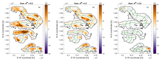
Figure 8 Dom model misfit ${\mathit{h}}^{\mathrm{true}}-{\mathit{h}}^{{\mathrm{est}}_k}$ after selected stages of the experimental design procedure using observed data (see also vertical dashed lines in Fig. 5). The selected GPR profiles are superimposed with green lines.

The profile associated with the largest discrepancy $d_{\mathrm{1}}^{\mathrm{cost}}$ is expected to offer the largest amount of additional information per unit cost. In this virtual experiment, we assumed that one would acquire this profile and subsequently perform a GlaTE inversion, yielding an improved model ${\mathit{h}}^{{\mathrm{est}}_k}$. Index k indicates the actual state of the experimental design, that is, k is equal to 1, when adding the first profile. Then, the next profile line to be acquired is identified using

$$\begin{array}{}\text{(15)}& d_{k+\mathrm{1}}^{\mathrm{cost}}=\underset{j}{max}\left({\displaystyle \frac{\sum _{\mathrm{i}=\mathrm{1}}^{i=n_j}P\left(\left|h_{ij}^{\mathrm{GPR}}-h_{ij}^{{\mathrm{est}}_k}\right|/h_{ij}^{\mathrm{GPR}}\right)}{c_j}}\right).\end{array}$$

Repeated application of Eq. (15) identifies an optimized sequence for how the profiles should be acquired. Figure 5a, c and e show the evolution of what we call the “data fit curve”, that is, the evolution of

$$\begin{array}{}\text{(16)}& d_{k+\mathrm{1}}^{\mathrm{fit}}={\displaystyle \frac{\sum _{j=\mathrm{1}}^{j=\mathrm{nprof}}\sum _{i=\mathrm{1}}^{i=n_j}\widehat{P}\left(\left|h_{ij}^{\mathrm{GPR}}-h_{ij}^{{\mathrm{est}}_k}\right|/h_{ij}^{\mathrm{GPR}}\right)}{\sum _{j=\mathrm{1}}^{j=\mathrm{nprof}}{n}_j}},\end{array}$$

with

$$\begin{array}{}\text{(17)}& \widehat{P}\left(x\right):=\left\{\begin{array}{ll}\mathrm{0}& \text{if }x>{\mathit{\epsilon }}^{\mathrm{GPR}}\\ \mathrm{1}& \text{if }x\le {\mathit{\epsilon }}^{\mathrm{GPR}}\end{array}\right.\end{array}$$

For the Vadret da Morteratsch data, there is an approximately linear increase in the data fit curve. Likewise, we observe a corresponding linear decrease in the average model misfit. As discussed in Maurer et al. (2010), cost–benefit curves, such as the d^fit graphs in Fig. 5, typically enter into the area of diminishing returns at some stage, that is, the curves exhibit a characteristic kink and flatten out at larger numbers of profiles. This indicates that it becomes increasingly expensive to obtain additional information. The curve in Fig. 5a therefore indicates that the area of diminishing returns was not reached during the Vadret da Morteratsch campaigns and that it would have been useful to acquire more profiles. In contrast, the d^fit and average misfit curves for the Glacier de la Plaine Morte and Dom regions (Fig. 5c and e) start flattening out, although we do not observe a characteristic kink in the curves. This indicates that it would have become increasingly expensive to obtain a more accurate ice thickness distribution for the Glacier de la Plaine Morte and Dom field sites.

Figures 6 to 8 show examples of model misfit plots $\left({\mathit{h}}^{{\mathrm{est}}_k}-{\mathit{h}}^{\mathrm{true}}\right)$ superimposed with the selected profile lines. The corresponding stages of the selection procedure are indicated with dashed black lines in Fig. 5a, c and e. For Vadret da Morteratsch, profiles are selected preferentially in the western part of the glacier because the model fit is already quite good in the eastern region. For the Glacier de la Plaine Morte and Dom regions, no obvious selection patterns can be recognized.

A major limitation of this design experiment is that the true model and the recorded GPR profiles have a strong dependency. When all profiles of a particular region are selected, there is a perfect match between ${\mathit{h}}_k^{\mathrm{est}}$ and h^true. However, this is the result of our choice of the true model, and thus it does not indicate that this data set is optimal.

To reduce this dependency at least partially, we have generated synthetic data sets that are covering all glacierized areas with a dense grid. We assumed a line spacing of 100 m and an inline sampling interval of 0.5 m, which is representative for the helicopter-borne GPR data that we acquired. With such a comprehensive data set, the experimental design procedure should have more flexibility to choose cost-optimized suites of profiles.

The resulting cost–benefit curves are shown in Fig. 5b, d and f. As expected, the curves start flattening out after selecting a sufficiently large number of profiles. For Vadret da Morteratsch (Fig. 5b), it seems to be worthwhile to acquire more than the 43 profiles acquired during the actual experiment. After about 70 profiles, the curve starts flattening out. The curves for Glacier de la Plaine Morte (Fig. 5d) indicate clearly that acquiring a larger number of profiles would have been beneficial. After adding about 40 profiles, the d^fit curve starts flattening out. For the Dom region, the amount of profiles chosen for the actual survey seems to be adequate (Fig. 5f). After approx. 40 profiles, the curve flattens out.

Figure 9 Vadret da Morteratsch model misfit ${\mathit{h}}^{\mathrm{true}}-{\mathit{h}}^{{\mathrm{est}}_k}$ after selected stages of the experimental design procedure using synthetic data (see also vertical dashed lines in Fig. 5). The selected GPR profiles are superimposed with green lines.

Using the d^fit curves in Fig. 5 seems to be a good option for selecting an appropriate number of profiles, but it is also insightful to consider the associated model misfit curves. Figure 5b, d and f indicate that the average thickness misfit typically approaches a low level before the d^fit curves start flattening out.

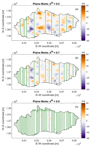
Figure 10 Glacier de la Plaine Morte model misfit ${\mathit{h}}^{\mathrm{true}}-{\mathit{h}}^{{\mathrm{est}}_k}$ after selected stages of the experimental design procedure using synthetic data (see also vertical dashed lines in Fig. 5). The selected GPR profiles are superimposed with green lines.

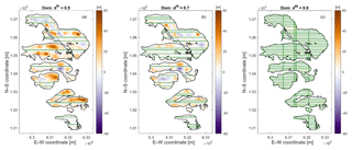
Figure 11 Dom Region model misfit ${\mathit{h}}^{\mathrm{true}}-{\mathit{h}}^{{\mathrm{est}}_k}$ after selected stages of the experimental design procedure using synthetic data (see also vertical dashed lines in Fig. 5). The selected GPR profiles are superimposed with green lines.

For the experimental design with the synthetic data, Figs. 9 to 11 show examples of model misfit plots $\left({\mathit{h}}^{{\mathrm{est}}_k}-{\mathit{h}}^{\mathrm{true}}\right)$ superimposed with the selected profile lines. In contrast to the selection based on observed data from the Vadret da Morteratsch (Fig. 6), the design based on the dense synthetic grid (Fig. 9) yields a better balance of profiles among the eastern and western portions of the glacier. This is the consequence of the larger flexibility of choosing profiles with the dense grid. For Glacier de la Plaine Morte (Fig. 10), it is interesting to note that almost exclusively N–S-oriented profiles were chosen. In contrast, predominantly E–W-oriented profiles were chosen for the Dom region (Fig. 11). Both observations are governed primarily by the cost factor c_j in Eq. (15).

4 Discussion and conclusions

The GlaTE inversion scheme presented in this paper offers numerous beneficial features. A benchmark for its capabilities, compared with other methods, will be evaluated in the framework of the ITMIX2 initiative, which is currently ongoing.

Its main advantage is its versatility, as there are several parameters by which the algorithm can be tuned to the peculiarities of a particular investigation area. However, this is also one of the method's major drawbacks, since the choice of the control parameters may include a considerable amount of subjectivity. This applies primarily to the choice of the weighting factors λ₁, λ₂ and λ₄. We consider our strategy for determining these factors to be adequate, but other options may work equally well.

Another potential problem is the determination of the scaling factor α_GPR in Eq. (7). It is largely dependent on the available GPR data, and it is assumed that the GPR profiles have a good areal coverage, which might not be always the case. If values for α_GPR become available for a large number of glaciers, a statistical analysis might be used to correlate the values with specific features of the glaciers (e.g., average slope, elevation above sea level, size or shape of the glacier, exposure, etc.). This may be helpful in areas where the GPR data coverage is poor or even nonexistent.

In principle, any observations (e.g., boreholes) can be employed as data constraints in Eq. (1), but GPR measurements are typically the main source of information. Migration of the GPR data allows the bedrock reflections to be imaged at the correct position and slope along a profile, but it is possible that the reflections originated from locations away from the profile lines (off-plane reflections). This may cause systematic errors affecting the reliability of the results. We note, however, that this is not a problem specific to GlaTE, but rather a general issue affecting GPR data acquired on a sparse grid.

As mentioned in Sect. 2, the system of equations in Eq. (11) can be augmented by any linear constraint. An obvious and, in our view, particularly useful set of constraints could be offered by surface displacement measurements. They can be obtained from differential satellite images and offer full coverage over a glacier. Such constraints could possibly substitute the smoothness constraints in Eq. (11) with a physically more meaningful quantity.

Despite the limitations of our experimental design approach, we judge that our results provided useful insights for designing GPR experiments and that some answers to the questions posed in Sect. 3 can be provided.

1. Was the experimental geometry and the amount of data acquired in the three investigation areas adequate?

   The cost–benefit curves in Fig. 5 indicate that, at least for Vadret da Morteratsch, it would have been useful to acquire more data.

2. Do better experimental layouts exist for constraining the ice thicknesses in a cost-optimized manner?

   The experimental layouts in Figs. 6 to 11 do not provide unexpected features but indicate that acquiring a larger number of shorter profiles, instead of recording a few long ones, could be beneficial, but it should be noted that we do not take into account the flight time required to move to the next profile. This could be significant on glaciers with steep mountain flanks.

3. Can some general recommendations for designing helicopter-borne GPR surveys on glaciers be made?

   Based on our results, it is difficult to offer general recommendations. For estimating the overall amount of data to be collected, the cost–benefit curves are most indicative. However, in our case studies they do not flatten out clearly, thereby indicating that it would be worthwhile to acquire more data. When high-precision ice thickness maps are required, it is therefore advisable to acquire as much data as can be afforded.

   It is common practice to acquire crossing profiles, but from the experimental layouts, shown in Fig. 10, it could be concluded that it is not necessary to acquire a large amount of crossing profiles. From a practical point of view, this recommendation cannot be fully supported. When the signal-to-noise ratio of the GPR profiles is poor, it can be difficult to identify the bedrock reflections unambiguously. Due to the importance of crossing profiles, it has been to be judged worthwhile to extend the cost function of the experimental design algorithm, such that crossing profiles are favored.

   It is not realistic to adopt a real-time experimental design strategy (i.e., choosing the next profile based on the results of the previously acquired data), as assumed in our virtual experiments in Sect. 3. However, if logistically feasible, it might be useful to employ a two-step acquisition strategy. Initially, only a few profiles could be acquired. After analyzing these data sets, regions where large discrepancies between h^est and h^glac exist can be identified and thus a suitable set of additional profiles could be acquired with a second campaign.